Week 4.2: Project - Transient simulation of flow over a throttle body

Aim: to setup and run the transient state simulation for flow over throttle body.

Geometry

• Import geometry
  
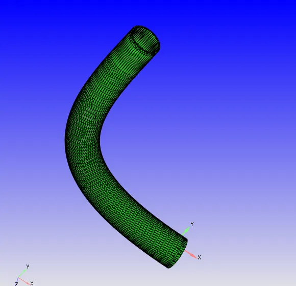
• extract the internal volume
  
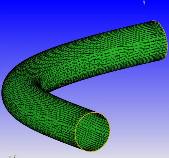
• Close the openings
  
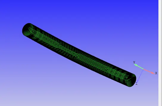
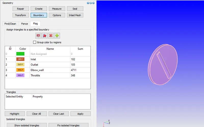
• Assign boundaries
  • Inlet
  • Outlet
  • Elbow wall
    
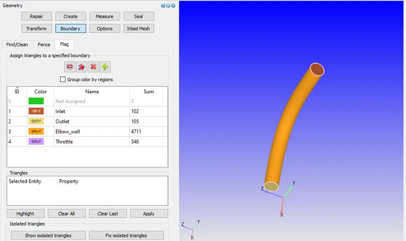
  • Throttle
    
• Check diagnostics
  
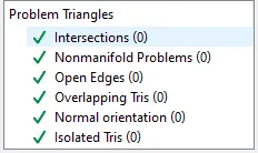
  Everything seems perfect as per diagnostic result.

Case setup

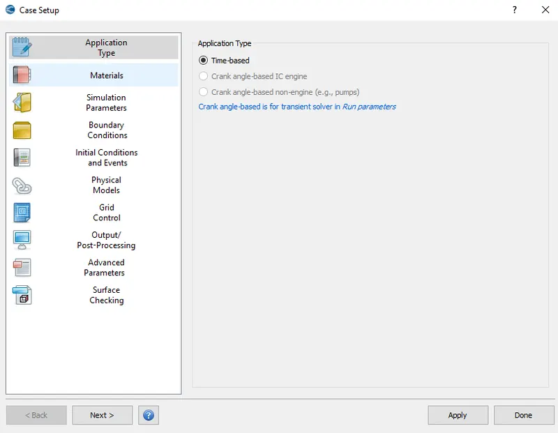
• Application type: Time based
  
  
• Materials
  gas simulation
  predefined mixture: Air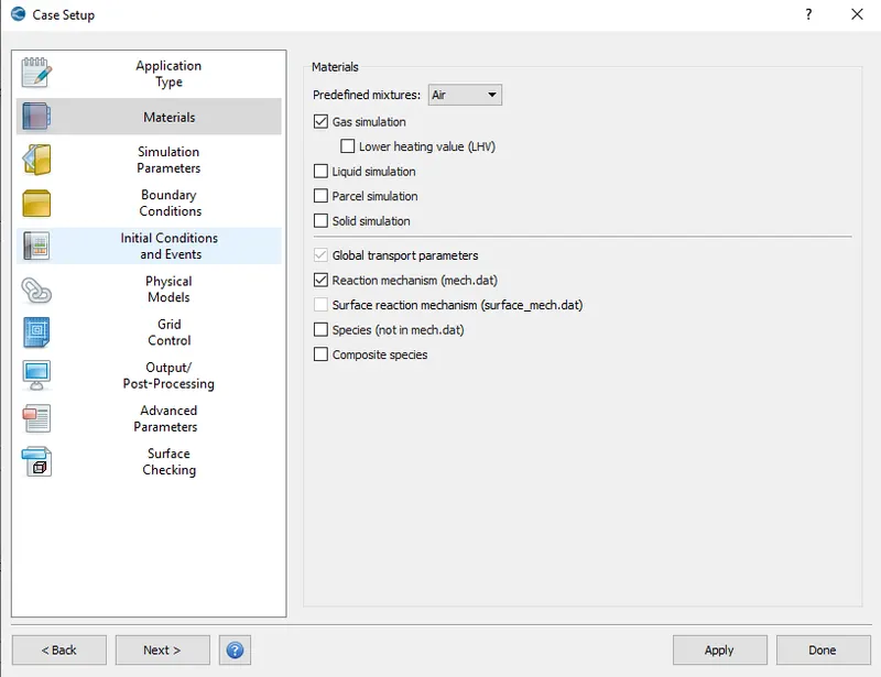
  
  
• Gas simulation
  Equation of state: Redich-Kwong
  Critical temperature: 133K
  Critical pressure: 3770000Pa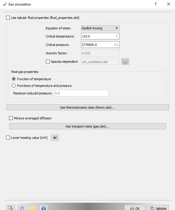
  
  
• Global transport properties
  turbulent Prandtl number: 0.9
  Turbulent Schmidt number: 0.8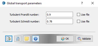
  
  
• Reaction mechanism
  Available species `O_2` and `N_2`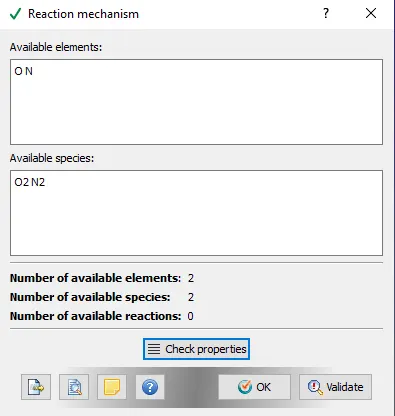
  
  
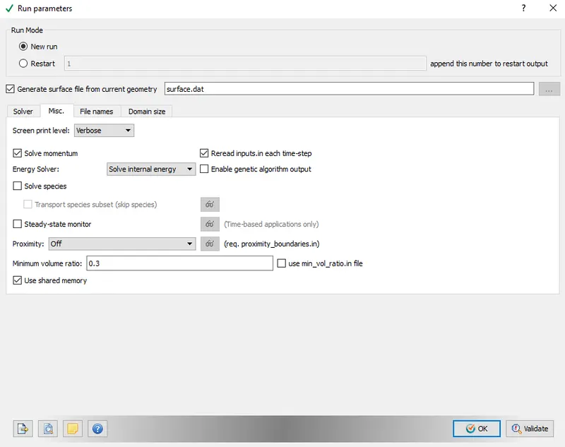
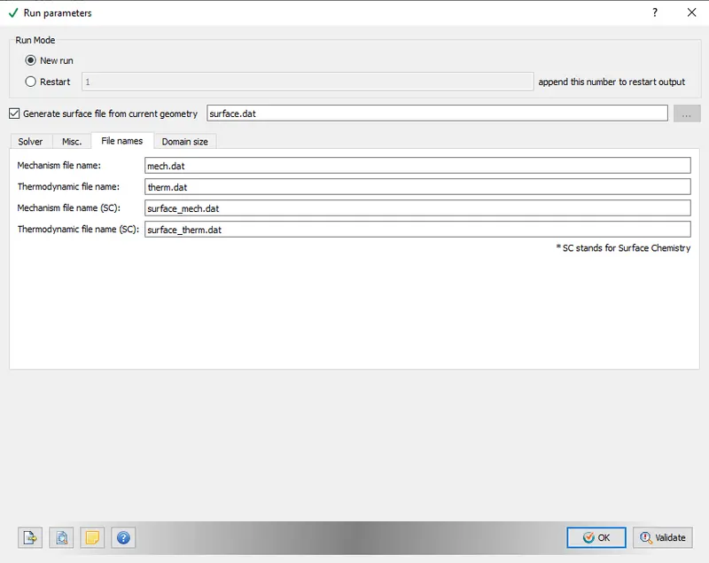
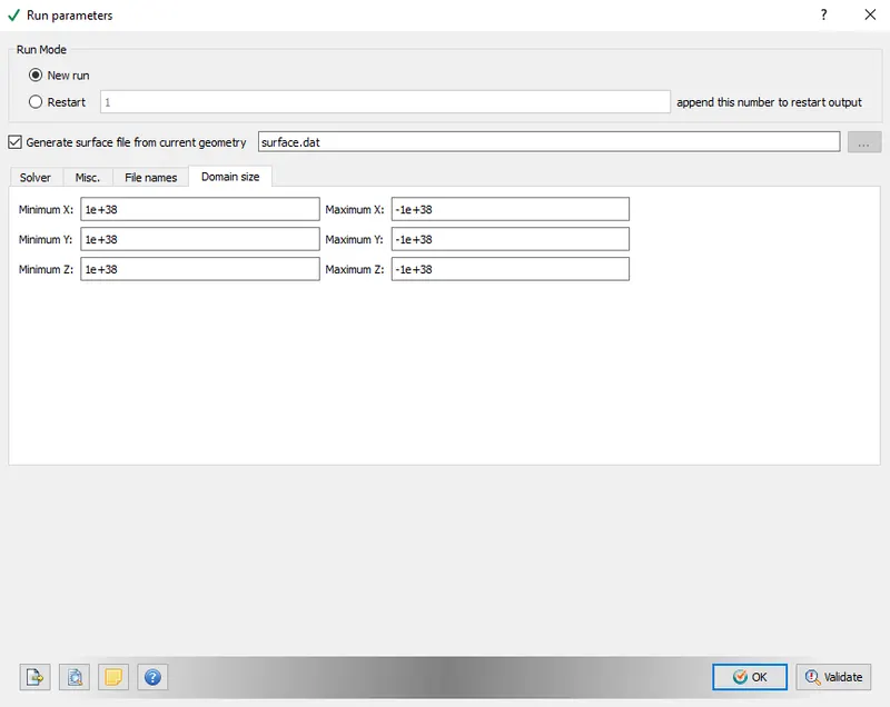
• Run parameters
  Solver: steady state
  Simulation mode: Full hydrodynamic
  Gas flow solver: Compressible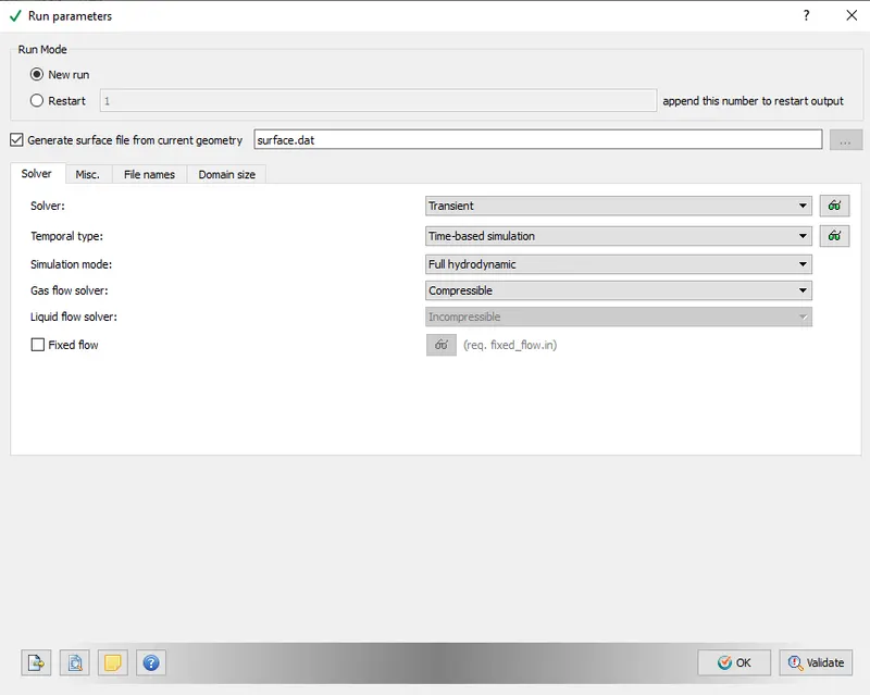
  
  
  
  
  
  
  
  
  
  

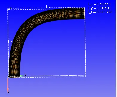
• Calculation of End time of simulation
  

  • • From the above contour we can say that length of pipe is approximately 0.2m
    • from steady state simulation we can say average velocity is = 170m/sec
    • speed = distance/time
      so, Time = 0.2/170sec
    • time = 0.001sec
    • for 10 cycles = 10*0.001=0.01sec
    • hence end time = 0.01sec
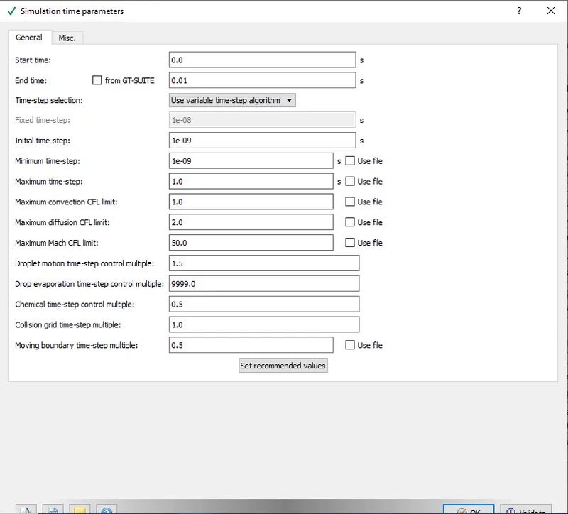
• Simulation time parameter
  • Start time par: 0 sec
  • end time: 0.01 sec
  • time step selection: use variable time-step algorithm
  • Initial time step: 1e-9Sec
  • Minimum time step: 1e-9sec
  • maximum time step: 1sec
    
    

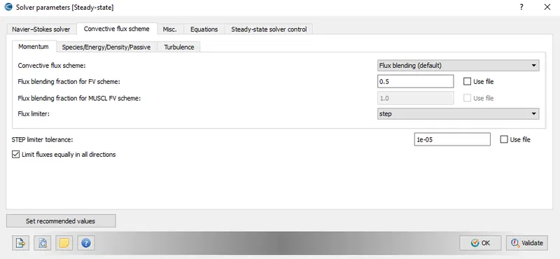
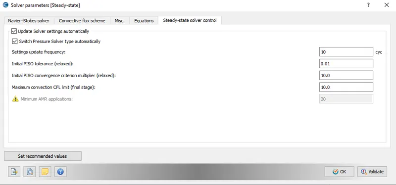
• Solver parameter
  Navier-stokes solver scheme: PISO
  Navier-stock solver type: pressure based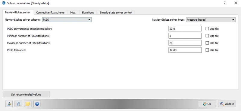
  
  
  
  
  
  
  
• Boundary
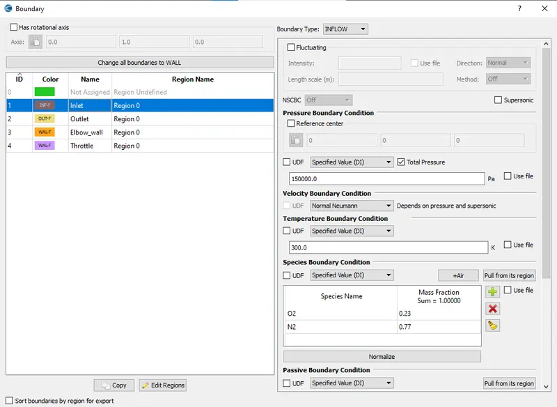
  • Inlet
    • Boundary type: INFLOW
    • Pressure: 150000Pa
    • Temperature: 300K
    • Species: `O_2` and `N_2`
      
      
  • Outlet
    
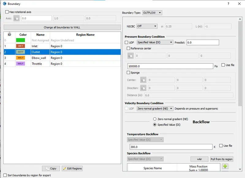
    • Boundary type: OUTFLOW
    • Pressure: 100000Pa
    • Temperature: 300K
    • Species: `O_2` and `N_2`
      
      
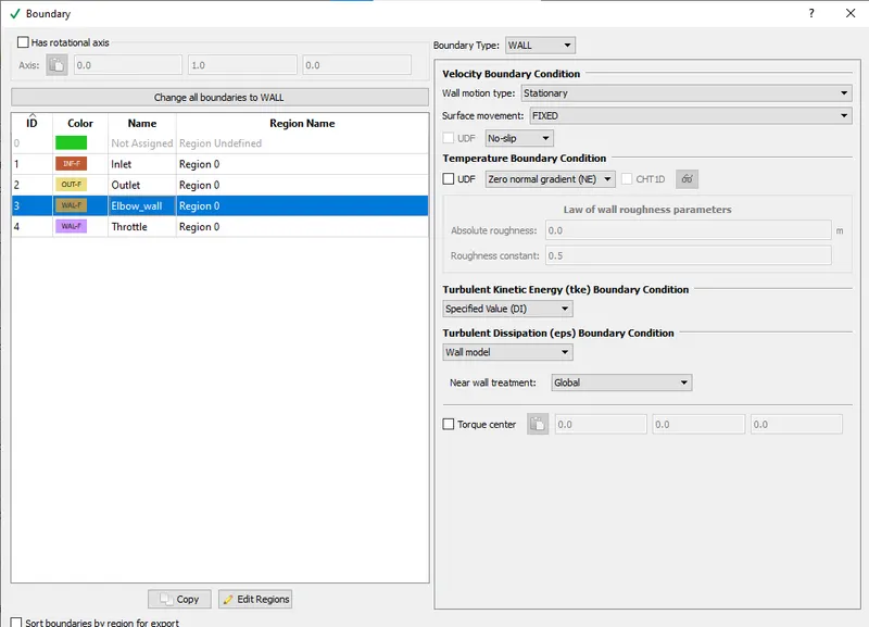
  • Elbow
    
    • Boundary type: wall
      
  • Throttle
    • Boundary type: wall
    • Wall motion type: Rotating
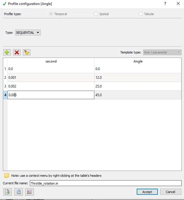
    • Setting up throttle rotation
      • at zero second = valve angle 0
      • at 0.001ms = 12 degree
      • at 0.002=25 degree
      • at 0.003ms = 45 degree
        

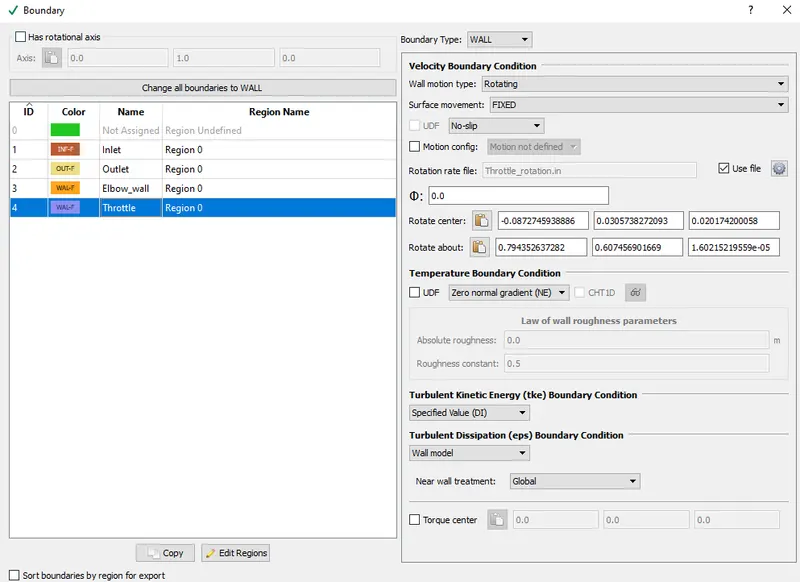
• Regions and initialization
  
  
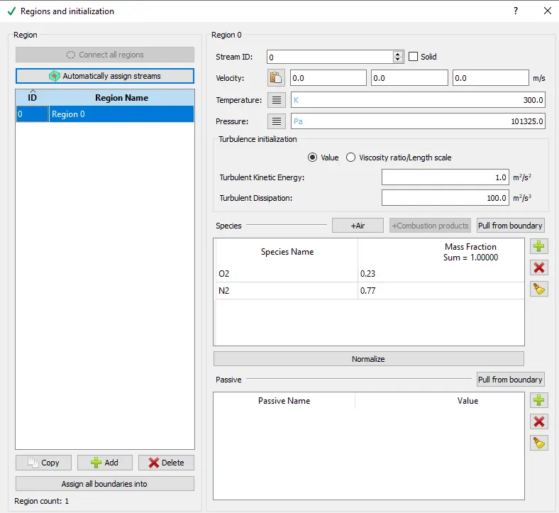
• Turbulence modelling
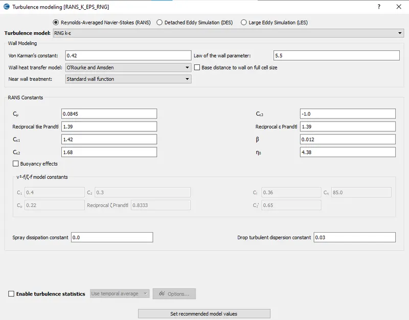
  • Turbulence model: RNG K-`epsilon`
    
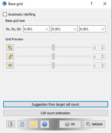
• Base grid
  • Grid size: 1mm
    
    
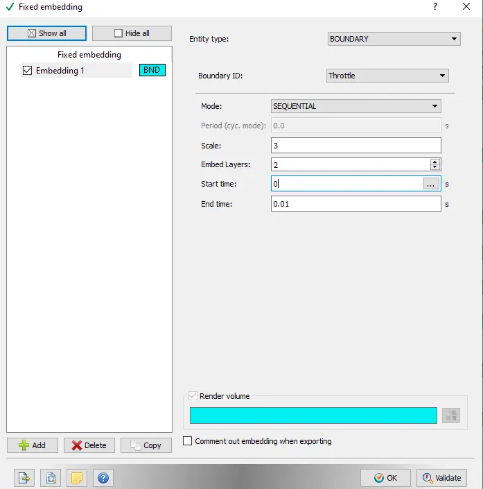
  • Fixed Embedding
    • Entity type: boundary
    • Boundary ID: Throttle
    • Mode: sequential
    • Scale:3
    • Embedded layers:2
    • Start time: 0sec
    • End time: 0.01sec
      
      
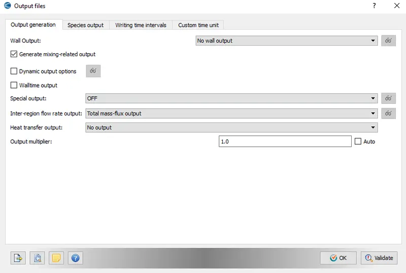
• Output files
  

Result and outputs

mass flow rate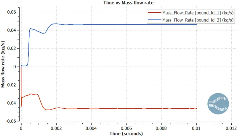

Average Mass flow rate at inlet is -0.045kg/sec and at outlet 0.045kg/sec. From the above plot we can conclude that simulation has converged approximately after 0.0035sec.

Average velocity

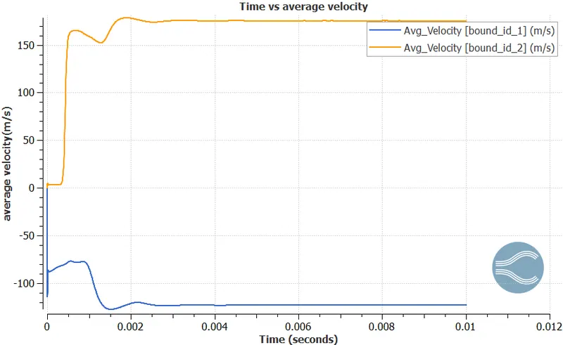
average velocity at inlet is -125m/sec and at outlet 175m/sec. From the above plot we can conclude that simulation has converged after 0.003sec.

Total pressure

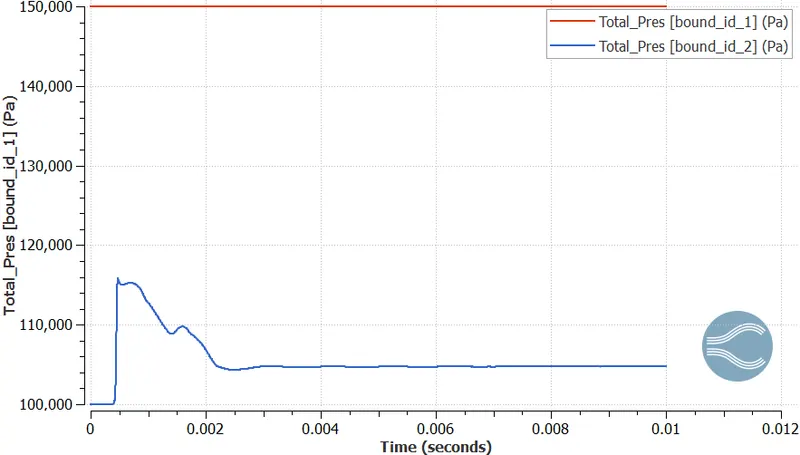
Total average pressure at the inlet is 150000 Pa and at outlet 105000 Pa. From the above plot we can conclude that simulation has converged after 0.003sec.

Total Cell count

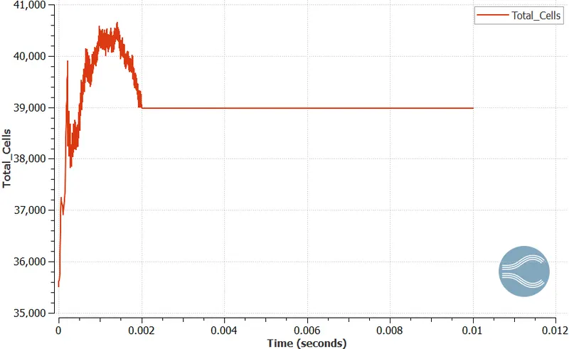
since we have enabled adaptive mesh refinement. That's why we are getting fluctuation in number of cells. upto 0.002 seconds valve is closing till 45 degrees. After that wall is stationary that's why we don't see any change in no. of cells.

Mesh

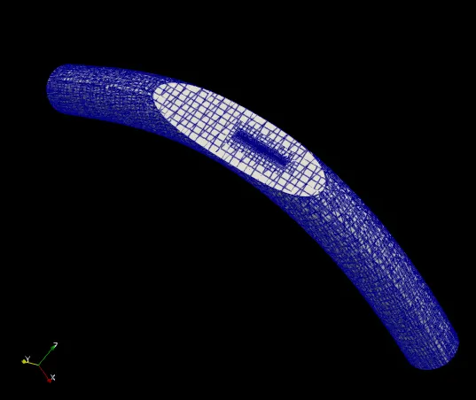
Since we have enabled adaptive mesh refinement near the throttle, we can observe the refined mesh near the throttle wall.

Velocity contour

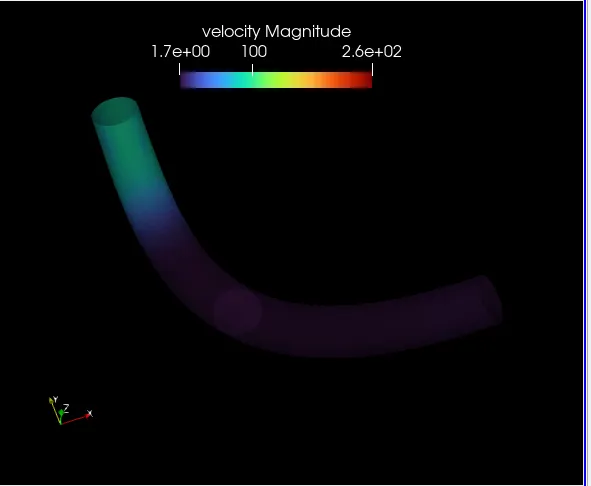
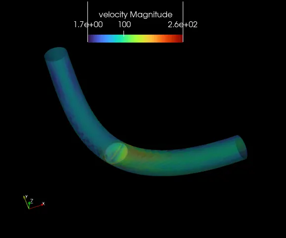
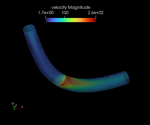
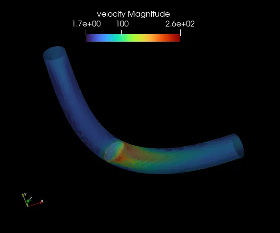
From the above contours we can observe that velocity around the throttle is higher because of minimum area of flow.

Pressure contour

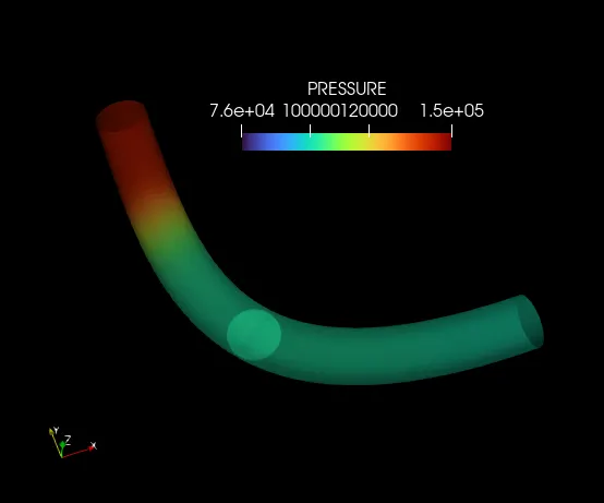
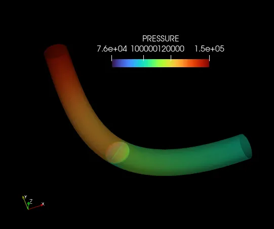
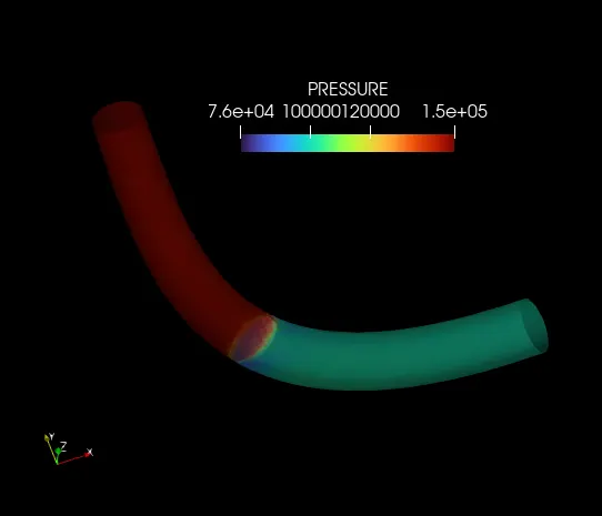
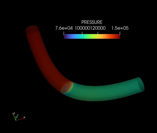
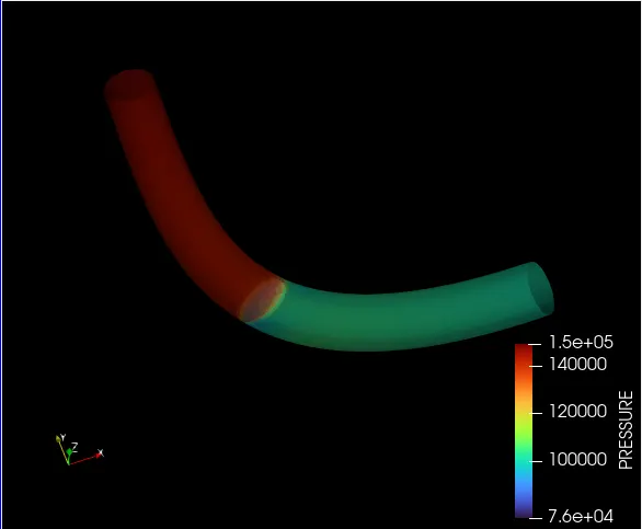
From the above pressure contour we can observe that pressure is gradually increasing in the elbow. but when the throttle closes 45 degrees. pressure behind the throttle becomes very low because of flow separation.

Pressure contour video link

https://youtu.be/BJN7JDsTKVQ

Velocity contour video link

https://youtu.be/zTiprdJmABY

Conclusion

• Velocity and pressure are higher at throttle from inlet side but lower at other side of the throttle because of flow separation is taking place which is causing wake region.
• From The mass flow rate plot, we can observe that mass flow rate at inlet is same as outlet so we can say that flow is steady state.
• Usually, we see a flat line in total cell throughout the simulation but in this case, we observe a deviation in cell count because of adaptive mesh refinement.