Week 4.2: Project - Transient simulation of flow over a throttle body

Aim:

To setup and simulate the Transient simulation of flow over throttle body.

l. INTRODUCTION

A throttle is a mechanism by which fluid flow is managed by constriction or obstruction. An engine's power can be increased or decreased by the restriction of inlet gases (by the use of a throttle), but usually decreased. The term throttle has come to refer, informally, to any mechanism by which the power or speed of an engine is regulated, such as a car's accelerator pedal.

ll. OBJECTIVE

• Simulate fluid flow over a throttle body using a transient state solver.
• Plot and analyze Velocity and Pressure Contours
• Plot and analyze Velocity, Pressure, Mass flow rate, total cell count.

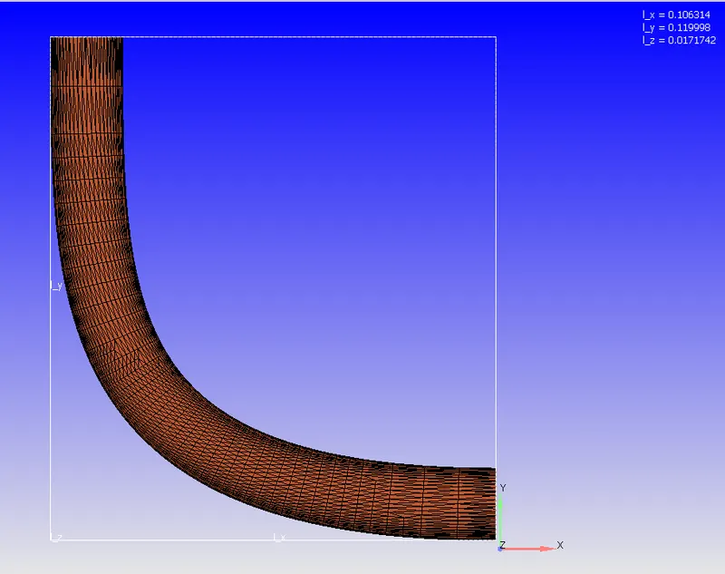
lll. GEOMETRY

The geometry consists of 4 basic components:

• Elbow Wall
• Inlet
• Outlet
• Throttle

1. Geometry Setup

Geometry setup in converge studio.

• Scaling the geometry - scaling the dimension of the cad model to meters.
• Removing all the open edges - closing the inlet & outlet open edge.

2. Diagnosis Check

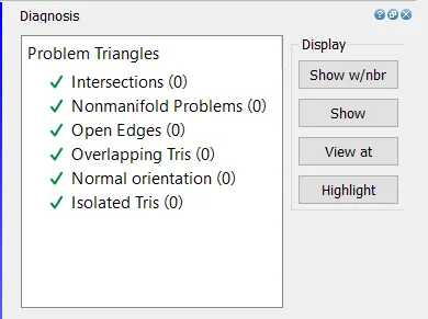
To check whether any error is present or not

3. Boundary Flagging

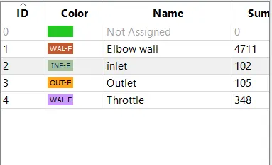
Combinig the boundary & assigning the proper names.

lV. Case Setup

1. Fluid: Air

Mass Fraction of Nitrogen: 0.77

Mass Fraction of Oxygen: 0.23

2. Solver:

A transient solver is used to simulate the flow.

3. Simulation Parameters:

The simulation end time can be approximated as follow:

The length of the elbow can be approximated using the characteristic length in the X and Y directions.

Length of the Elbow =sqrt((0.1062)+(0.122))=0.16≈0.2(0.1062)+(0.122)=0.16≈0.2 m

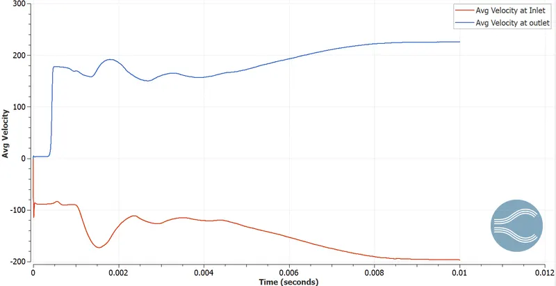
Velocity at the Inlet (as obtained in the steady-state simulation) = 190 m/s

Flow time = 0.2/190 = 0.001052 ≈≈ 0.002 s

The fluid should flow at least three to four times through the entire elbow.

Total Flow time =0.002 x 4 =0.008 s

The end time is taken slightly greater than the approximated time.

End Time = 0.01 s

Simulation Time Parameters:

Start Time: 0 s

End Time: 0.01 s

Initial time-step: 1e-9 s

Minimum Time-step: 1e-9 s

Maximum time-step: 1 s

4. Boundary Conditions:

• Elbow Wall: Boundary Type - Wall | Velocity Boundary Condition - Law of Wall
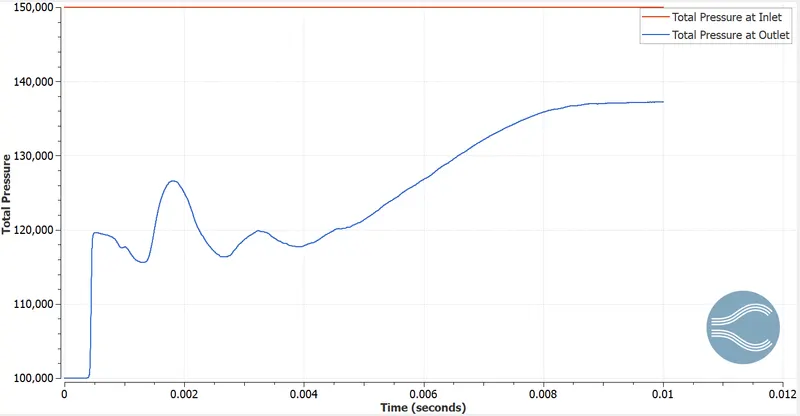
• Inlet: Boundary Type - INFLOW | Total Pressure = 150000 Pa | Temperature = 300 K | Species = Air
• Outlet: Boundary Type - OUTFLOW | Static Pressure = 100000 Pa | Temperature = 300 | Species = Air
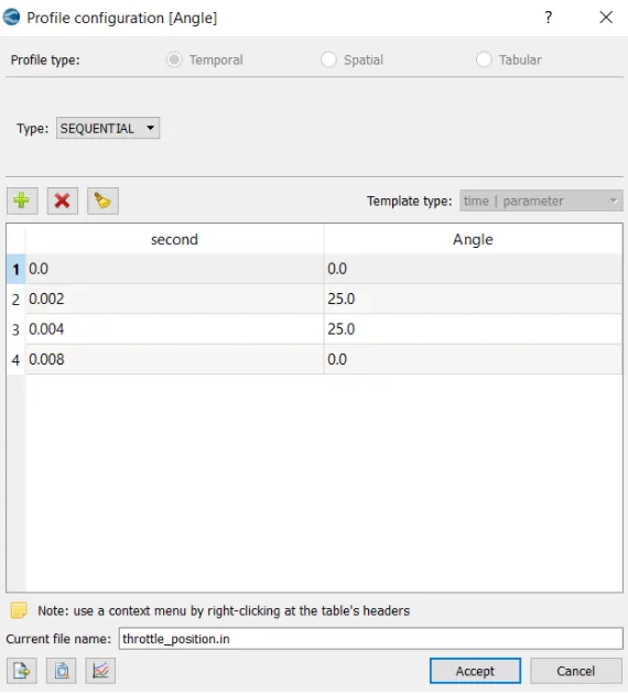
• Throttle: Boundary Type - WALL | Wall Motion Type - Rotating | Surface Movement - Moving | Velocity Boundary Condition - Law of Wall
  
  Rotation Rate File:
• From 0 to 2 ms the valve should rotate by 25 degrees.
• From 2 to 4 ms ut should stay at 25 degrees.
• After which by 8 ms the valve should get back to its original position

5. Regions and Initialization:

• Flow Region: Volumetric Flow Region
• Total Pressure: 101325 Pa
• Temperature: 300 K
• Species: Air

6. Turbulence Model: RNG k-epsilon

7. Grid Control:

Base Grid:

• dx=dy=dz= 2e-3 m
  
  Fixed Embedding:
  
• Entity Type: Boundary
• Boundary ID: Throttle
• Mode: Permanent
• Scale: 3
• Embed Layers: 2

8. Output Files:

The time interval for writing 3-D output files will depend on the number of the outputs desired by the user. In this case, we will take 80 outputs.

Number of Outputs = 80

Time interval for writing 3-D output files= Simulation Time/ Number of Outputs = 0.01/80 = 0.000125 s

Writing Time Intervals

• The time interval for writing 3-D output files: 0.000125 s
• The time interval for writing text output: 1e-6 s
• The time interval for writing restarting output: 0.001 s

V. RESULTS

1. Mesh

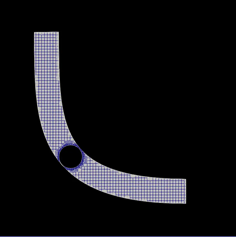
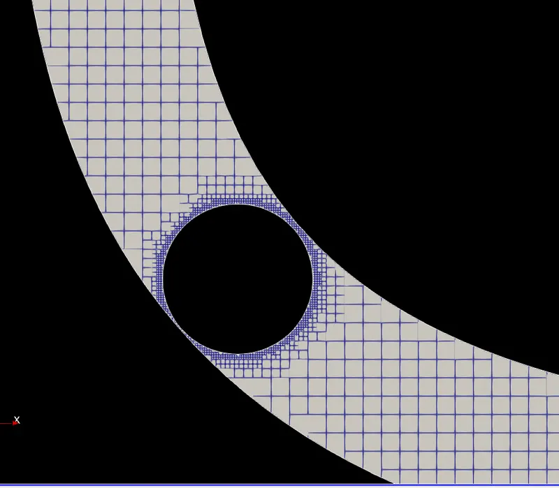
Decreasing the mesh size around the throttle helps capture the results at the throttle boundary more accurately and results in the smoothening of the contours around the throttle. However, this also increases the computation time due to the increased number of cells.

Mesh

Mesh around the Throttle

2. Velocity Contours and Pressure Contours

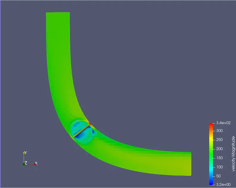
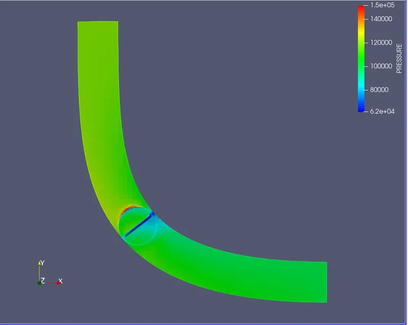
As the valve closes, the velocity of the fluid decreases. This also results in a sudden increase in the pressure in the region behind the throttle as, kinetic energy gets converted into pressure energy.

Velocity Contour

Pressure Contour

3. Velocity Vectors

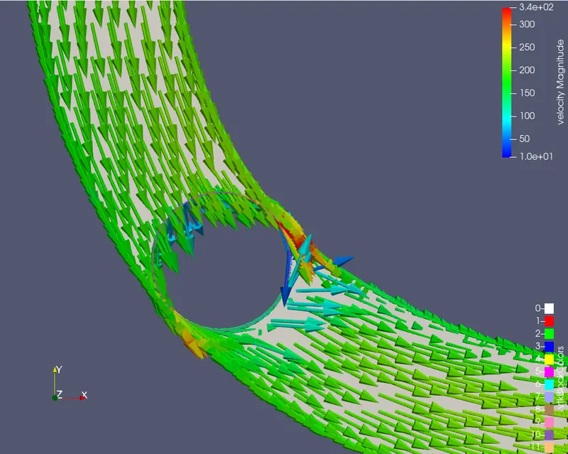
The velocity contour can be understood by observing the direction of flow using velocity vectors.

Velocity Vectors

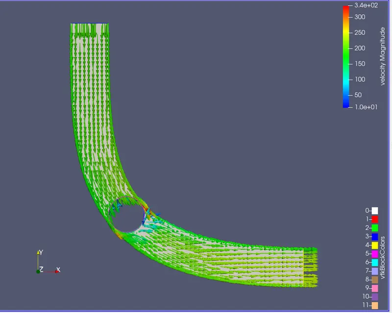
Velocity Vectors around the Throttle

4.Velocity Streamlines

The velocity streamlines represent the direction in which a mass less fluid element will travel at any point in time. A lot of disturbances are created which can be analyzed using the velocity streamlines which occurs during the small rotation of the valve.

5. Variation of Average Velocity w.r.t. Time

6. Variation of Pressure w.r.t. Time

7. Variation of Mass Flow Rate w.r.t. Time

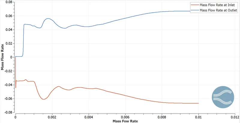
The mass flow rate at the inlet is equal to the negative of the mass flow rate at the outlet at the end of the simulation. This shows that the mass flow is conserved.

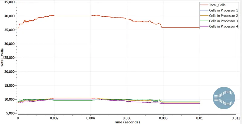
8. Variation of Cells Count w.r.t. Time

Velocity Contour

https://drive.google.com/file/d/1PTie-RfToROYdeoymsAZjM9XovzJHWzL/view?usp=sharing

Pressure Contour

https://drive.google.com/file/d/1y6vfDFL0Rzb1mtWmrkfKepMDEGjzPbgA/view?usp=sharing

There is almost even distribution of cells among the 4 processors to obtain a load balance, as simulation is simple.

Since the throttle is moving, the number of cells near the throttle changes to adapt to the movement of the throttle.

As the mesh generated along the throttle position is refined that is by providing 2 embedded layers & a scaling of 3 to the mesh, the flow through the throttle position is more accurate.

As we have a mobile mesh, number of cells generated are more, therefore simulation time is high.

Conclusion:-

The behavior of the fluid helps us to understand & control the flow & the throttle movement such that we get the required output without any disturbances.

Various plots, contours are generated to study the flow over a throttle body.