Week 4.1 - Solving second order ODEs

Aim:

Write a program in Matlab that will simulate the pendulum motion

Theory:

The 2nd Order ODE represents many Engineering problems and arriving to solution of 2nd ODE gives a better insights to study the engineering systems.

For example:

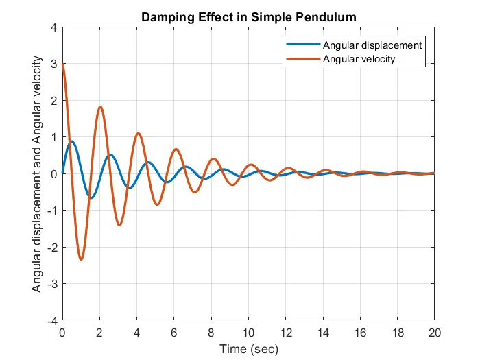
Motion of simple pendulam is represented as 2nd Order ODE.The solution of equation will help us to study the relationship between the displacement and velocity variation with respect to mass,damping co eff and length.

program code:

%Second Order ODE of a Simple Pendulum and its Animation
clear all
close all
clc

%Inputs
b = 0.5;     %damping coefficient
g = 9.81;     %acceleration due to gravity in m/s2
l = 1;        %length of the pendulum in m
m = 1;        %mass of the pendulum bob in kg

%Initial condition
theta_0 = [0;3];

%Time span
t_span = linspace(0,20,600);

%Solving ODE
[t,y] = ode45(@(t,theta) ode_func(t,theta,b,g,l,m),t_span,theta_0);

%Plotting Angular displacement and Angular velocity w.r.t Time
plot(t,y(:,1),'linewidth',2);
hold on;
plot(t,y(:,2),'linewidth',2);
axis([0 20 -4 4]);
xlabel('Time (sec)');
ylabel('Angular displacement and Angular velocity');
grid on
title('Damping Effect in Simple Pendulum');
legend('Angular displacement','Angular velocity');
pause(10);

ct = 1;
for i = 1:length(t_span);    
    x0 = 0;
    y0 = 0;
      
    x1 = l*sin(y(i,1));
    y1 = -l*cos(y(i,1));
    
    %Simulation of motion of Pendulum
    plot([x0 x1],[y0 y1],[-0.5 0.5],[0 0],'linewidth',3)
    hold on 
    plot(x1,y1,'marker','o','markerSize',25,'markerFacecolor','r')
    axis([-1.5 1.5 -1.5 0.5])
    grid on
    title('Motion of a Simple Pendulum with Damping')
    pause(0.01)
    M(ct) = getframe(gcf);
    ct=ct+1;
    hold off
end

%Animation of motion of Simple Pendulum
movie(M)
videofile = VideoWriter('Simple_Pendulum.avi','Uncompressed AVI')
open(videofile)
writeVideo(videofile,M)
close(videofile)

function [dtheta_dt]=ode_func(t,theta,b,g,l,m)
theta1=theta(1)
theta2=theta(2)
dtheta1_dt=theta2;
dtheta2_dt=-(b/m)*theta2-(g/l)*sin(theta1);
dtheta_dt=[dtheta1_dt;dtheta2_dt];
end

output plot: