Week 4.1 - Solving second order ODEs

AIM: To write a program in Matlab that will simulate the pendulum motion.

GOVERNING EUATIONS: To solve the ODE funtion the governing equation which is used are

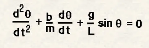
OBJECTIVE OF PROJECT: To make a MATLAB code which can give solution of second order differently equations in details and to plot the graph for the same and animation of the second order.

BODY OF CONTENT: Below is the function code of ODE.

function [dtheta_dt] = ode_func(t,theta,b,g,l,m)

theta1 = theta(1)
theta2 = theta(2)
dtheta1_dt = theta2;
dtheta2_dt = -(b/m)*theta2-(g/l)*sin(theta1);
dtheta_dt = [dtheta1_dt;dtheta2_dt]
end

This code is used to call the function which is dreived in the equation.

Now below is the main code of ODE for ploting and animation.

clear all
close all
clc

b=0.05;
g=9.81;
l=1;
m=0.1;

% initial condition
theta_0=[0;3];
% time points
t_span=linspace(0,20,500);

% solve ODE
[t,results]=ode45(@(t,theta) ode_func(t,theta,b,g,l,m),t_span, theta_0);
plot(t,results(:,1))
hold on
plot(t,results(:,2))
xlabel('time');
ylabel('Plot');
% creating animation
ct=1;
for i=1:500;

    x0=0;
    y0=0;
    x1=l*sin(results(i,1));
    y1=-1*cos(results(i,1));
    figure(2);
    plot([-0.5 0.5],[y0 y0],'LineWidth',10);
   axis([-1.5 1.5 -1.5 1.5]);
    grid on
    hold on
    line([x0 x1],[y0 y1],'linewidth',2,'color','r');
    plot(x1,y1,'o','markersize',20,'MarkerFaceColor','r');
    hold off
    title('damping of pendulum');
    legend('support rod','ball of pendulum','length of pendulum');
    M(ct)=getframe(gcf);
    ct=ct+1;
end
%creating movies
movie(M)
videofile = VideoWriter('simple_pendulum.avi','Uncompressed AVI');
open(videofile);
writeVideo(videofile,M)
close(videofile);

The above code gives the time plot for the ode function as shown below

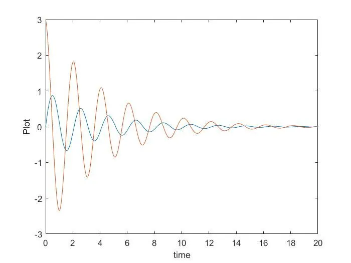
and for the animation video here is the link of simple pendulum.

https://youtu.be/YXNOpeN8cCI

CONCLUSION:.

The simple motion of pendulum as been acheived by these code in MATLAB.