Week 4.1 - Solving second order ODEs

Aim :

To solve a 2nd Order Differential Equation of a simple pendulum using MATLAB.

Objective :

• To write a program to solve the ODE of the motion of a simple pendulum using MATLAB.
• Plot the graph of the displacement and velocity.
• Create a simulation of the pendulum in motion.

Description:

The motion of a simple pendulum is an example of simple harmonic motion, consisting of a small bob and a massless string. Movement of the pendulum depends on Newton's second law. When this law is written down, a second-order Ordinary Differential Equation is formed that describes the position of the end of the pendulum w.r.t time.

This linear equation helps us in understanding different engineering phenomenon and principles. Here we shall consider the motion of a simple pendulum through a 2nd Order Differential Equation.

Equation of motion is:

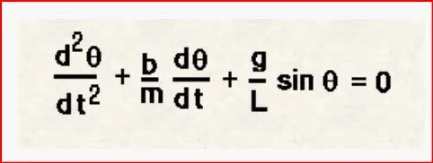
In the above equation,

• g = gravity in m/s^2.
• L = length of the pendulum in the meter.
• m = mass of the ball in kg.
• b = damping coefficient.

Since the given function is in the second-order differential equation we will convert it into first order to solve the ODE.

     Let
                θ=θ1

                dθ1/dt=θ2

                dθ^2/dt^2=dθ2/dt

Input :

       b = damping coefficient.

       m = mass of the bob in Kg.

       g = the gravity in m/s^2.

       l = length of the string in m.

Matlab main Code 

%program to simulate the transient behaviour of a simple pendulum
clear all
close all
clc

%inputs
b = 0.05;   %damping coefficient
g = 9.81;   %Acceleration due to gravity
l = 1;      %Length of Pendulum in meters
m = 1;      %Mass 


% initial condition
theta_0 = [0;4];

% time points
t_span = linspace(0,30,500);

% solve ODE
[t, results] = ode45(@(t,theta) ode_func(t,theta,b,g,l,m),t_span, theta_0);

% ploting
plot(t,results(:,1))
hold on
plot(t,results(:,2))
ylabel('Plot')
xlabel('Time in sec')

% Iteration using for loop to create animation of simple pendulum
ct=1;
theta_1 = results(:,1);

for i= 1:length(results(:,1))
    
    % initial co-ordinates
    x_start= 0;
    y_start= 0;
    theta_2 = theta_1(i);
    
    % final co-ordinates
    x_end = 1*sin(theta_2);
    y_end = -1*cos(theta_2);
    
    % ploting for animation
    figure(2)
    % base of pendulum
    plot([-1,1],[0,0], 'linewidth',8,'color','green')
    hold on
    % string of pendulum
    line([x_start x_end],[y_start y_end],'linewidth',5,'color','b')
    hold on
    % bob of pendulum
    plot(x_end,y_end,'marker','o','markersize', 35,'markerfacecolor','r')
    axis([-2 2 -2 2])
    pause(0.03)
    hold off
    M(ct)=getframe(gcf)
    ct=ct+1;
end
% creating movie from captured frames
 movie(M)
 videofile = VideoWriter('simple_pendulum.avi','uncompressed AVI');
 open(videofile);
 writeVideo(videofile,M);
 close(videofile);

Function code 

function [dtheta_dt] = ode_func(t,theta,b,g,l,m)
        
         theta1 = theta(1)
         theta2 = theta(2)
         dtheta1_dt = theta2;
         dtheta2_dt = -(b/m)*theta2 - (g/l)*sin(theta1);
         dtheta_dt = [dtheta1_dt; dtheta2_dt];
end

Explanation 

•  In the first step Input and initial condition [0;4]; of a simple pendulum are fed.
•  Then the program is written to solve the ODE in which Matlab inbuilt function (ode45) is used with constant theta, t, and another function is used, which is defined separately in function program.

• The ODE is integrated in order to obtain the solution. The time span is defined using a linear spaced array, t_span = linspace (0,30,500); where the time is taken between 0 to 20 seconds.

  ode45 is an inbuilt solver in MATLAB used to integrate differential equations. To solve the differential equation we use an anonymous function. 

•  In the next step result of solved ODE is plotted w.r.t time using plot command.
•  Now iteration of co-ordinate is fed using for loop to create animation.
• Then plot command is used to plot pendulum string and bob.
•  In the next step, the move command is used to create an animated video of the oscillating pendulum.

 Error:

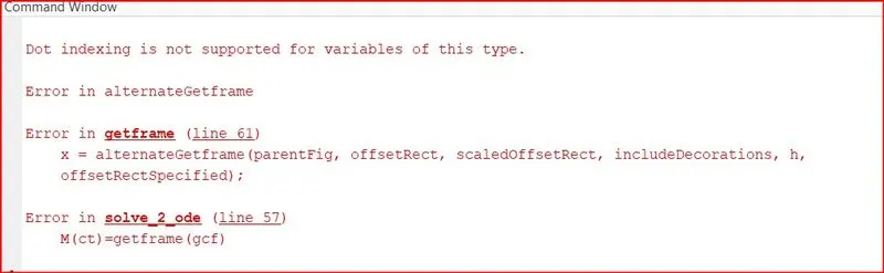
the animation was interupted below completing 500 instances as given,therefore error resolved by running the program upto 500 instances.Hence the output animation is completed.

Output Result of the matlab code 

 Plot : 

 

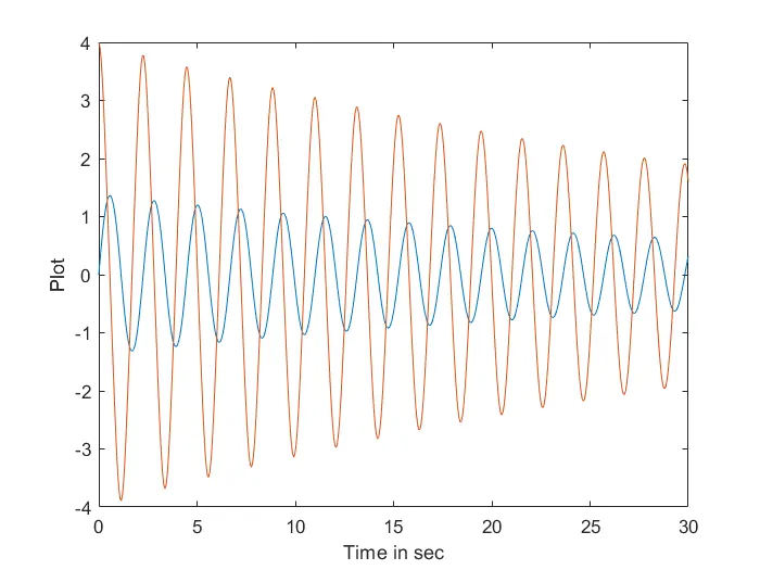
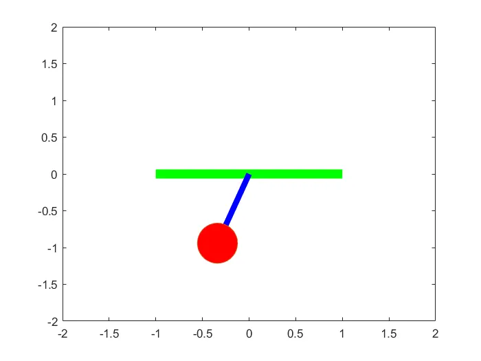
 Animation link of the simple pendulum 

         https://youtu.be/b0ncqHDvWZ4

Conclusion 

Created  the 2nd Order Differential equation of a pendulum in motion using MATLAB with the solution we were able to plot a graph of the oscillation of the pendulum and a video of the pendulum in motion.

NOTE: The matlab code files with (.m) extention has been sunmitted below 

Thankyou