Week 4.1 - Solving second order ODEs

Aim:

To develop a Matlab program to solve the second-order ordinary differential equation governing the motion of a damped pendulum, incorporating parameters such as gravity, pendulum length, mass, and damping coefficient. Utilize the solution to simulate the pendulum's motion over a specified time interval and visualize its dynamic behavior through animation.

Objective:

The objective of this MATLAB code is to simulate and animate the motion of a damped simple pendulum using ordinary differential equations. Equations are formulated to include damping effects, considering factors such as gravity, length, mass, and damping coefficient. Numerical methods are utilized to compute the angular displacement and velocity of the pendulum across a designated time span. The program leverages MATLAB's capabilities to generate an animation illustrating the pendulum's dynamic behavior. This task showcases the application of ODEs in engineering for simulating and visualizing real-world systems.

Problem Statement:

When illustrating the transient behaviors exhibited by various systems, ordinary differential equations (ODEs) are extensively employed in engineering. A simple pendulum serves as a prime example of this concept, as its motion adheres to Newton's second law of motion. By solving the motion equation using MATLAB, individuals can explore the functionality of MATLAB's numerical integration capabilities, such as the ode45 solver. This hands-on approach facilitates comprehension of the essential parameters required for precise numerical integration and resolution of differential equations in this context. Figure 4 represents the main parameters that need to be considered to characterize the motion of a simple pendulum.

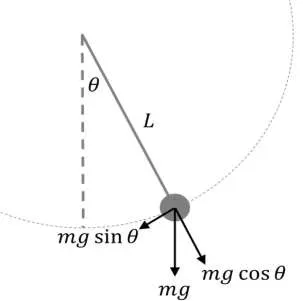
Figure 4: The motion of a simple pendulum.

Equations Used:

The second order differential equation coupled with the arrangement in matrix form:

`(d^2theta)/(dt) + b/m (d theta)/dt + g/l sintheta = 0`

Where,

𝜽 is the angular displacement; 𝒃 is the damping coefficient; 𝒎 is the mass of the bob; 𝒈 is the acceleration due to gravity; 𝒍 is the length of the pendulum

Assuming that `theta = theta_1` and `(d theta_1)/dt = theta_2`, and solving ODE in matrix form:

`d/dt((theta_1),(theta_2)) = ((theta_2),(-b/mtheta_2 - g/l sintheta_1))`

Matlab Program:

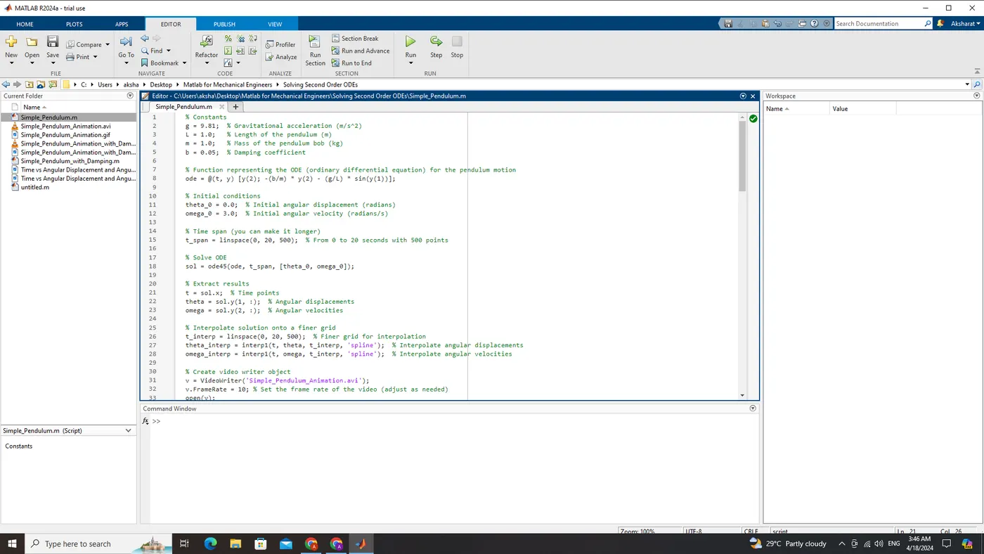
% Constants
g = 9.81;  % Gravitational acceleration (m/s^2)
L = 1.0;   % Length of the pendulum (m)
m = 1.0;   % Mass of the pendulum bob (kg)
b = 0.05;  % Damping coefficient

% Function representing the ODE (ordinary differential equation) for the pendulum motion
ode = @(t, y) [y(2); -(b/m) * y(2) - (g/L) * sin(y(1))];

% Initial conditions
theta_0 = 0.0;  % Initial angular displacement (radians)
omega_0 = 3.0;  % Initial angular velocity (radians/s)

% Time span (you can make it longer)
t_span = linspace(0, 20, 500);  % From 0 to 20 seconds with 500 points

% Solve ODE
sol = ode45(ode, t_span, [theta_0, omega_0]);

% Extract results
t = sol.x;  % Time points
theta = sol.y(1, :);  % Angular displacements
omega = sol.y(2, :);  % Angular velocities

% Interpolate solution onto a finer grid
t_interp = linspace(0, 20, 500);  % Finer grid for interpolation
theta_interp = interp1(t, theta, t_interp, 'spline');  % Interpolate angular displacements
omega_interp = interp1(t, omega, t_interp, 'spline');  % Interpolate angular velocities

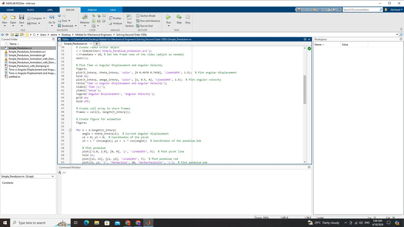
% Create video writer object
v = VideoWriter('Simple_Pendulum_Animation.avi');
v.FrameRate = 10; % Set the frame rate of the video (adjust as needed)
open(v);

% Plot Time vs Angular Displacement and Angular Velocity
figure;
plot(t_interp, theta_interp, 'color', [0 0.4470 0.7410], 'LineWidth', 1.5);  % Plot angular displacement
hold on;
plot(t_interp, omega_interp, 'color', [1, 0.5, 0], 'LineWidth', 1.5);  % Plot angular velocity
title('Time vs Angular Displacement and Angular Velocity');
xlabel('Time (s)');
ylabel('Value');
legend('Angular Displacement', 'Angular Velocity');
grid on;
hold off;

% Create cell array to store frames
frames = cell(1, length(t_interp));

% Create figure for animation
figure;

for i = 1:length(t_interp)
    angle = theta_interp(i);  % Current angular displacement
    x1 = 0; y1 = 0;  % Coordinates of the pivot
    x2 = L * sin(angle); y2 = -L * cos(angle);  % Coordinates of the pendulum bob
    
    % Plot pendulum
    plot([-2.0, 2.0], [0, 0], 'y', 'LineWidth', 5);  % Plot pivot line
    hold on;
    plot([x1, x2], [y1, y2], 'LineWidth', 3);  % Plot pendulum rod
    plot(x2, y2, 'o', 'MarkerSize', 20, 'MarkerFaceColor', 'w');  % Plot pendulum bob
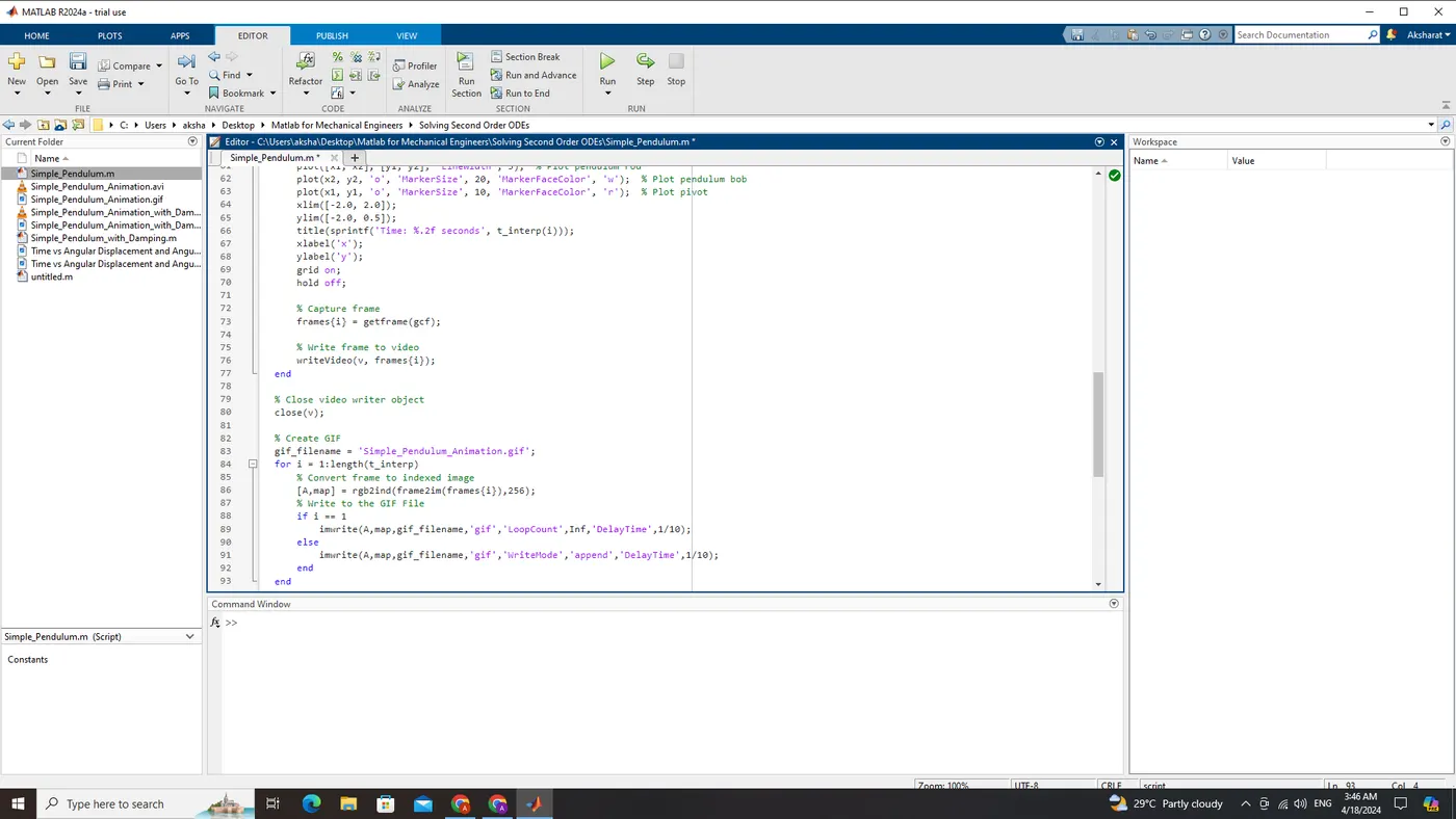
    plot(x1, y1, 'o', 'MarkerSize', 10, 'MarkerFaceColor', 'r');  % Plot pivot
    xlim([-2.0, 2.0]);
    ylim([-2.0, 0.5]);
    title(sprintf('Time: %.2f seconds', t_interp(i)));
    xlabel('x');
    ylabel('y');
    grid on;
    hold off;
    
    % Capture frame
    frames{i} = getframe(gcf);
    
    % Write frame to video
    writeVideo(v, frames{i});
end

% Close video writer object
close(v);

% Create GIF
gif_filename = 'Simple_Pendulum_Animation.gif';
for i = 1:length(t_interp)
    % Convert frame to indexed image
    [A,map] = rgb2ind(frame2im(frames{i}),256);
    % Write to the GIF File
    if i == 1
        imwrite(A,map,gif_filename,'gif','LoopCount',Inf,'DelayTime',1/10);
    else
        imwrite(A,map,gif_filename,'gif','WriteMode','append','DelayTime',1/10);
    end
end

Explanation:

Constants and Function Definition

% Constants
g = 9.81;  % Gravitational acceleration (m/s^2)
L = 1.0;   % Length of the pendulum (m)
m = 1.0;   % Mass of the pendulum bob (kg)
b = 0.05;  % Damping coefficient

% Function representing the ODE (ordinary differential equation) for the pendulum motion
ode = @(t, y) [y(2); -(b/m) * y(2) - (g/L) * sin(y(1))];

In this section, physical constants such as gravitational acceleration, length of the pendulum, mass, and damping coefficient are defined. Additionally, the function ode is created to represent the ordinary differential equation governing the motion of the pendulum. This function describes how the angular displacement and velocity of the pendulum change over time.

Initial Conditions and Time Span

% Initial conditions
theta_0 = 0.0;  % Initial angular displacement (radians)
omega_0 = 3.0;  % Initial angular velocity (radians/s)

% Time span (you can make it longer)
t_span = linspace(0, 20, 500);  % From 0 to 20 seconds with 500 points

Here, the initial conditions for the pendulum are specified, including the initial angular displacement and velocity. Additionally, a time span is defined over which the simulation will run, from 0 to 20 seconds with 500 time points.

Solving the ODE

% Solve ODE
sol = ode45(ode, t_span, [theta_0, omega_0]);

This section employs the ode45 solver to numerically solve the ordinary differential equation defined earlier. It integrates the system of differential equations over the specified time span, starting from the initial conditions provided.

Extracting Results and Interpolation

% Extract results
t = sol.x;  % Time points
theta = sol.y(1, :);  % Angular displacements
omega = sol.y(2, :);  % Angular velocities

% Interpolate solution onto a finer grid
t_interp = linspace(0, 20, 500);  % Finer grid for interpolation
theta_interp = interp1(t, theta, t_interp, 'spline');  % Interpolate angular displacements
omega_interp = interp1(t, omega, t_interp, 'spline');  % Interpolate angular velocities

Here, the results from the solver are extracted. The time points, angular displacements, and angular velocities are obtained. Then, these results are interpolated onto a finer grid using interp1 to create smoother plots and animations.

Creating Video Writer Object and Plotting

% Create video writer object
v = VideoWriter('Simple_Pendulum_Animation.avi');
v.FrameRate = 10; % Set the frame rate of the video (adjust as needed)
open(v);

% Plot Time vs Angular Displacement and Angular Velocity
figure;
plot(t_interp, theta_interp, 'color', [0 0.4470 0.7410], 'LineWidth', 1.5);  % Plot angular displacement
hold on;
plot(t_interp, omega_interp, 'color', [1, 0.5, 0], 'LineWidth', 1.5);  % Plot angular velocity
title('Time vs Angular Displacement and Angular Velocity');
xlabel('Time (s)');
ylabel('Value');
legend('Angular Displacement', 'Angular Velocity');
grid on;
hold off;

This section initializes a video writer object to save the animation as a video file. It also plots the angular displacement and angular velocity over time, providing visual insights into the pendulum's motion.

Creating Cell Array for Frames and Animation Loop

% Create cell array to store frames
frames = cell(1, length(t_interp));

% Create figure for animation
figure;

for i = 1:length(t_interp)
    angle = theta_interp(i);  % Current angular displacement
    x1 = 0; y1 = 0;  % Coordinates of the pivot
    x2 = L * sin(angle); y2 = -L * cos(angle);  % Coordinates of the pendulum bob
    
    % Plot pendulum
    plot([-2.0, 2.0], [0, 0], 'y', 'LineWidth', 5);  % Plot pivot line
    hold on;
    plot([x1, x2], [y1, y2], 'LineWidth', 3);  % Plot pendulum rod
    plot(x2, y2, 'o', 'MarkerSize', 20, 'MarkerFaceColor', 'w');  % Plot pendulum bob
    plot(x1, y1, 'o', 'MarkerSize', 10, 'MarkerFaceColor', 'r');  % Plot pivot
    xlim([-2.0, 2.0]);
    ylim([-2.0, 0.5]);
    title(sprintf('Time: %.2f seconds', t_interp(i)));
    xlabel('x');
    ylabel('y');
    grid on;
    hold off;
    
    % Capture frame
    frames{i} = getframe(gcf);
    
    % Write frame to video
    writeVideo(v, frames{i});
end

In this part, a cell array called frames is created to store each frame of the animation. Then, a loop iterates over each time point in the interpolated time array t_interp. For each time point, it calculates the coordinates of the pendulum bob based on the current angular displacement. It then plots the pendulum components (pivot, rod, and bob) on a figure, updates the title to display the current time, and captures the frame using getframe. Each frame is added to the frames array and written to the video file using writeVideo.

Closing Video Writer Object

% Close video writer object
close(v);

After the animation loop, the video writer object v is closed to finalize the video writing process.

Creating GIF

% Create GIF
gif_filename = 'Simple_Pendulum_Animation.gif';
for i = 1:length(t_interp)
    % Convert frame to indexed image
    [A,map] = rgb2ind(frame2im(frames{i}),256);
    % Write to the GIF File
    if i == 1
        imwrite(A,map,gif_filename,'gif','LoopCount',Inf,'DelayTime',1/10);
    else
        imwrite(A,map,gif_filename,'gif','WriteMode','append','DelayTime',1/10);
    end
end

Finally, a GIF is created from the frames stored in the frames array. Each frame is converted to an indexed image, and then written to the GIF file using imwrite. The GIF filename is specified as "Simple_Pendulum_Animation.gif", and the delay time between frames is set to 1/10 seconds.

Output:

Simple_Pendulum

Simple Pendulum Animation

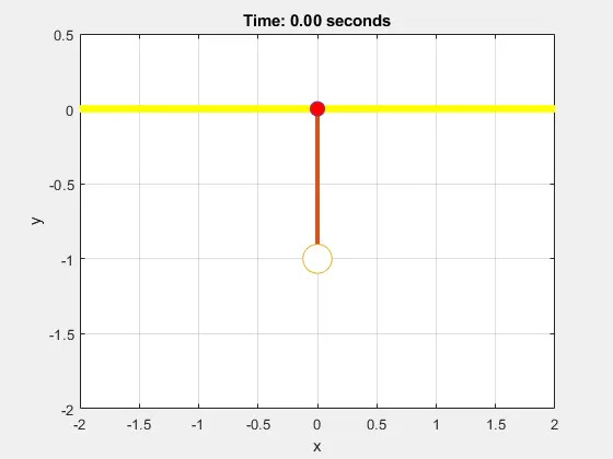
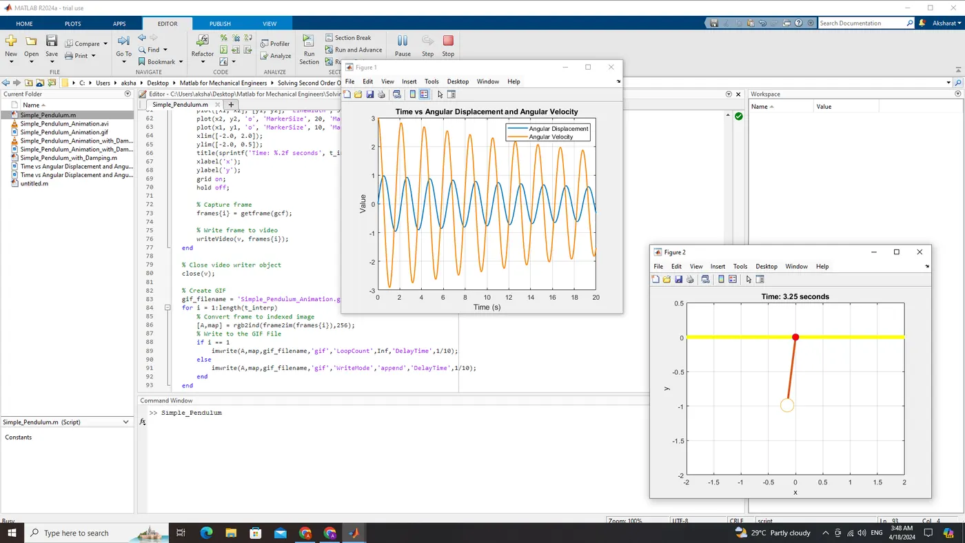
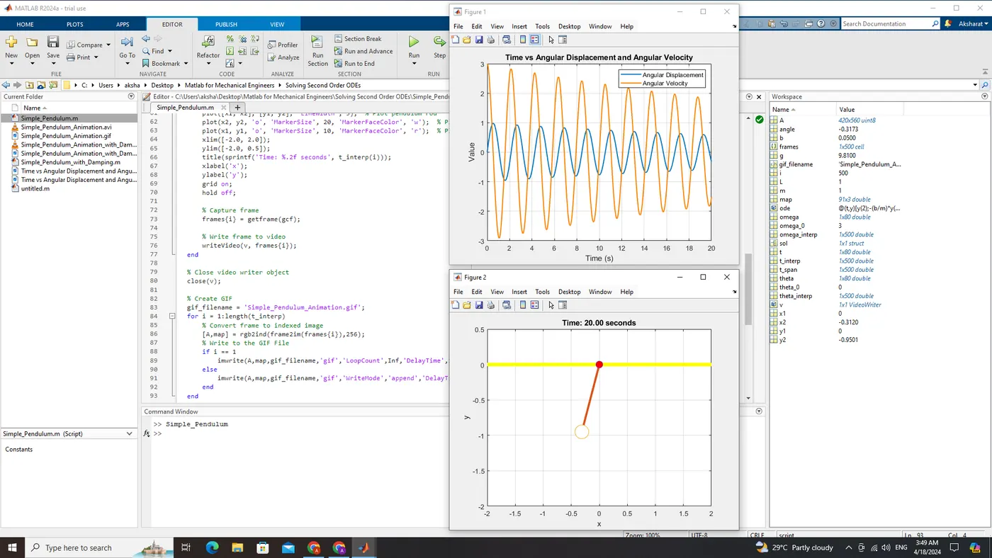
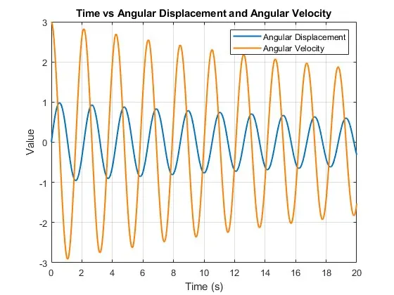
The output of the provided code is an animation that visually represents the motion of a simple pendulum over time, as well as plots showing the angular displacement and angular velocity of the pendulum.

Let's break down the output in detail:

1. Animation:

   • The animation visually displays the movement of a simple pendulum, where a mass (the pendulum bob) is attached to the end of a rod (the pendulum arm) and swings freely under the influence of gravity.
   • The pendulum bob swings back and forth, exhibiting oscillatory motion.
   • The animation starts with the pendulum at rest (initial position), and as time progresses, the pendulum bob swings back and forth due to the gravitational force acting on it.
   • Each frame of the animation shows the position of the pendulum bob at a specific time interval. The animation gives a clear representation of the dynamics of the pendulum motion.

2. Plots:

   • Two plots are generated:
     • Time vs. Angular Displacement: This plot shows how the angular displacement of the pendulum changes over time. It represents the angle between the pendulum arm and the vertical axis.
     • Time vs. Angular Velocity: This plot illustrates how the angular velocity of the pendulum changes over time. It represents the rate of change of angular displacement with respect to time.
   • Both plots provide insights into the dynamics of the pendulum motion. The angular displacement plot shows the oscillatory behavior of the pendulum, while the angular velocity plot gives information about how quickly the pendulum is swinging at different points in time.

In summary, the output of the code provides both visual and numerical representations of the motion of a simple pendulum, allowing for a comprehensive understanding of its behavior over time.

Conclusion:

The code efficiently simulates the motion of a simple pendulum and provides insightful visualizations through animation and plots. It accurately represents the pendulum's behavior over time, aiding in the understanding of oscillatory motion principles. The generated video (AVI) and GIF files offer accessible formats for sharing and dissemination of the results. Overall, the code serves as a valuable educational resource for studying pendulum dynamics and has practical applications in fields such as physics, engineering, and robotics.

Extras:

I have attached another ZIP file (Simple Pendulum with Damping) with the same code of the original zip file (Simple Pendulum), but the parameter of damping co-efficient is changed to "b = 0.5".

By changing the damping coefficient to "b = 0.5", the damping effect increases. This means that the pendulum experiences a stronger resistance against its motion, leading to quicker dissipation of its energy.

(It also has the files for GIF, AVI and Plot JPEG's along with Matlab Code File.)