Week 4.1 - Solving second order ODEs

 Aim:To solve second order oridinary differential equation using MATLAB.

Therory:

Ordinary Differential Equations(ODEs) -An ordinary differential equation (ODE) is a differential equation containing one or more functions of one independent variable and the derivatives of those functions.The term ordinary is used in contrast with the term partial differential equation which may be with respect to more than one independent variable.

ODE is used to describe the transient behavior of a system.A simpe example is a pendulum. The way pendulum moves depends on the Newtons second law. When this law is written down, we get a second order ordinary Differential Equation that desribes the position of the 'ball' w.r.t  time.

g=gravity in m/s^2

L==r=length of pendulum in m

m=mass of the ball in kg,

b=damping coefficient.

To write a program that solves the following ODE. This ODE reperesents the equation of motion of simple pendulum with a damping step hence solve it.

`d^2theta/dt^2+b/m*d theta/dt+g/l*sin theta`

Fundamental ODE function

`theta1=theta2`

`d theta/dt=theta2`

`d^2 theta/dt^2=d^2theta_1/dt^2=d/dt(d theta_1/dt)=d(theta_2)/dt`

`d^2 theta_1/dt^2+b/m*d theta_1/dt+g/l*sin theta_1`

`d theta_2/dt+b/m * theta_2+g/l sin theta_1`

`d theta_2/dt=-b/m*theta_2-g/l sin theta_1`

`d/dt [[theta_1],[theta_2]]=[[theta_2],[-b/m*theta_2-g/sin theta_1]]`

Explaination of code:

Main code:

clear all
close all
clc
b=0.05
g=9.81
L=1
m=0.1

%intial condition
theta_0=[0;3];
%time points
t_span=linspace(0,10,600);

[t,results]=ode45(@(t,theta)ode_func(t,theta,b,g,L,m),t_span,theta_0)

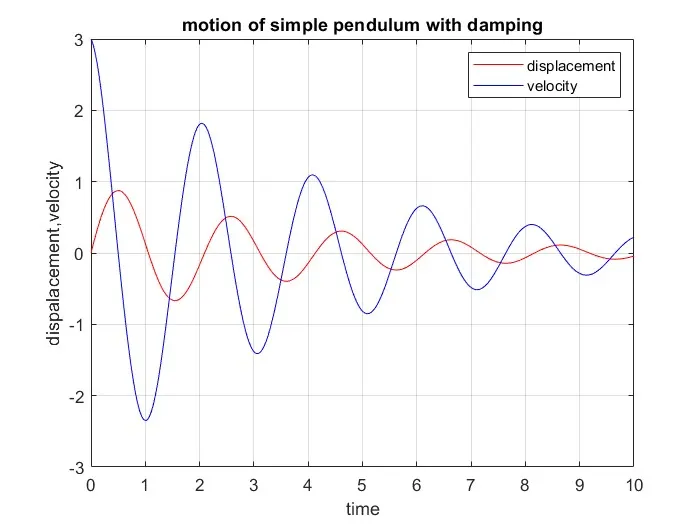
plot(t,results(:,1),'Color','r')
hold on
plot(t,results(:,2),'color','b')
xlabel('time')
ylabel('dispalacement,velocity')
legend('displacement','velocity')
title('motion of simple pendulum with damping')
grid on

%Animation
x0=0
y0=0

ct=1 %counter represent each and every frame
 for i=1:length(t)
     x1=L*sin(results(i,1))
     y1=-L*cos(results(i,1))
 figure(2)
 plot([-1 1],[0 0],'LineWidth',5,'Color','g')
 axis([-2 2 -2 2])
 line([x0 x1],[y0 y1],'linewidth',5,'color','b')
 hold on
 plot(x0,y0,'s','MarkerSize',5,'MarkerFaceColor','y')
 plot(x1,y1,'o','MarkerSize',25,'MarkerFaceColor','r')
 title('damping of simple pendulum')
 legend('support rod','length of pendulum','fixed point','Bod of pendulum')
 grid on
 hold off
 pause(0.1)
 M(ct)=getframe(gcf)
 ct=ct+1;

 end
 movie(M)
 videofile=VideoWriter('forward_kinetics_avi','Uncompressed AVI')
 open(videofile)
 writeVideo(videofile,M)
 close(videofile)

 Explanation:

• 'b=0.05', 'g=9.81', 'L=1', 'm=0.1':Define the constants for the the system -damping coefficient(b), gravitational acceleration(g), length of pendulum(L), and mass of the pendulum bob(m).
• theta_0=[0;5]: Set the intial conditions for the system. The penulum start from an angle of 0 radians and angular velocity of 5 rad/s.
• t_span=linspace(0,10,500): Create a vector 't_span' containing 500 equally spaced time points between 0 to 10 seconds.
• Solve the ordinary differential equations(ODEs) using the ode45 solver. The ODE function is defined in 'ode_func', taking time 't' , state 'theta', and the constants as inputs.
• Plots the first column of the 'results' matrix (angle) against time with red line.
• Holds the current plots so that subsequent plots are overlaid.
• Plots the second column of the 'results' matrix (angular velocity) aganist time with blue line.
• Add a lbel to the x and y axis.
• %animation
• Intial position of pendulum bob.
• Counter for frams in the animation.
• Loop through each time step.
• end the loop.
• Display the animation using the frame stored in 'M'.
• Creates a videoWriter object named 'forward_kinetics_avi' for uncompressed AVI format.
• Opens the video file for writing.
• Write the frames in 'M' to the video file.
• Closes the video file.

Function:

function[dtheta_dt]=ode_func(t,theta,b,g,L,m)
theta1=theta(1)
theta2=theta(2)
%velocity
dtheta1_dt=theta2
%accelerates=(-b/m)*(theta(2))-(g/L)*sin(theta(1))
dtheta2_dt=-(b/m)*theta2-(g/L)*sin(theta1)
dtheta_dt=[dtheta1_dt;dtheta2_dt]

 Explanation:

• First, all the input variables are assigned respective values as specified in problem.
• The function open_func available at the end of the code takes the input variables along with dependent variables (theta_1 and theta_2) and returns the ODE in the from of system of first -order differential equations.
• Finally, the respective arguments (function handle to ode_fun function, the time span and intial condition vector) are passed to the ode45 solver to finally obtain the solution of the differential equation in t and result matrices.
• The solver returns angle(theta_1) and angular velocity (theta_2) as the output in the results vector at each time point corresponding to value stored in the vector.

 Results:

 Link:

https://drive.google.com/file/d/1sk5EUzqbCqtkfbC9yoYLQoc7wOjuocma/view?usp=sharing