Week 4.1 - Solving second order ODEs

AIM:- write a program that solves the following ODE. This ODE represents the equation of motion of a simple pendulum with damping

GIVEN DATA

In the above equation,

g = gravity in m/s2,

L = length of the pendulum in m,

m = mass of the ball in kg,

b=damping coefficient.

Write a program in Matlab\Octave that will simulate the pendulum motion, just like the one shown in the start of this challenge.

use,

L=1 metre,

m=1 kg,

b=0.05.

g=9.81 m/s2.

Simulate the motion between 0-20 sec, for angular displacement=0,angular velocity=3 rad/sec at time t=0.

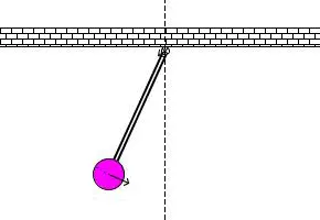
When you do this you will get the position of the pendulum as a function of time. Use this information to animate the motion of the pendulum, as shown in the below figure.

OBJECTIVES:- TO COMPLETE ALL TASK GIVEN ABOVE

PROGRAM:- CODING IN MATLAB

clear all
close all
clc

%Inputs
b = 0.05;     %damping coefficient
g = 9.81;     %acceleration due to gravity in m/s2
l = 1;        %length of the pendulum in m
m = 1;        %mass of the pendulum bob in kg

%Initial condition
theta_0 = [0;3];

%Time span
t_span = linspace(0,20,600);

%Solving ODE
[t,y] = ode45(@(t,theta) ode_func(t,theta,b,m,g,l),t_span,theta_0);

%Plotting Angular displacement and Angular velocity w.r.t Time
plot(t,y(:,1),'linewidth',2);
hold on;
plot(t,y(:,2),'linewidth',2);
axis([0 20 -4 4]);
xlabel('Time (sec)');
ylabel('Angular displacement and Angular velocity');
grid on
title('Damping Effect in Simple Pendulum');
legend('Angular displacement','Angular velocity');
pause(10);

ct = 1;
for i = 1:length(t_span);    
    x0 = 0;
    y0 = 0;
      
    x1 = l*sin(y(i,1));
    y1 = -l*cos(y(i,1));
    
    %Simulation of motion of Pendulum
    plot([x0 x1],[y0 y1],[-0.5 0.5],[0 0],'linewidth',3)
    hold on 
    plot(x1,y1,'marker','o','markerSize',25,'markerFacecolor','r')
    axis([-1.5 1.5 -1.5 0.5])
    grid on
    title('Motion of a Simple Pendulum with Damping')
    pause(0.01)
    M(ct) = getframe(gcf);
    ct=ct+1;
    hold off
end

%Animation of motion of Simple Pendulum
movie(M)
videofile = VideoWriter('Simple_Pendulum.avi','Uncompressed AVI')
open(videofile)
writeVideo(videofile,M)
close(videofile)

FUNCTION CODE

function [dtheta_dt] = ode_func(t,theta,b,m,g,L) % creating function named ode_func
  theta1=theta(1); % Assign value theta(1) to theta1
  theta2=theta(2); % Assign value theta(2) to theta2
  
  % find derivatio of theta1 and theta2
  dtheta1_dt = theta(2); 
  dtheta2_dt = -(b/m)*theta2-(g/L)*sin(theta1);
  
  % creating array of dtheta_dt for function which is coloumn matrix
  [dtheta_dt] = [dtheta1_dt; dtheta2_dt];
  
end

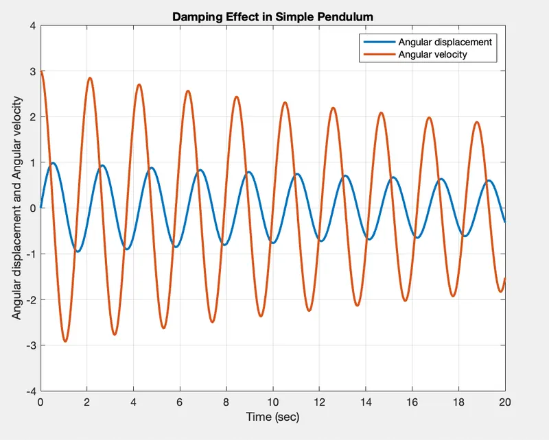
RESULTS :

COMMANDS USED

• CLOSES ALL :- closes all figures whose handles are visible.

• CLEAR ALL: - clear removes all variables from the current workspace, releasing them from system memory

• CLC :- clc clears all the text from the Command Window, resulting in a clear screen.

• FOR LOOP :- For loop control statements, you can repeatedly execute a block of code.

• Add Legend :-Add a legend to the graph that identifies each data set using the legend function. Specify the legend descriptions in the order that you plot the lines. Optionally, specify the legend location using one of the eight cardinal or intercardinal directions, in this case .

• Line width:- Itis used to adjust (increase) the width of any object. Line width operation mostly executes inside the plot operation. Plot operation is used to plot the input and output in a graphical way. We can increase the width of an object to any extent. By default, the line width size is ‘1’ in Matlab.
• COLORS :-The eight basic colors are known by either their short name or long name (RGB triplets are also included).

Long Name	Short Name	RGB Triplet
blue	b	[0,0,1]
black	k	[0,0,0]
red	r	[1,0,0]
green	g	[0,1,0]
yellow	y	[1,1,0]
cyan	c	[0,1,1]
magenta	m	[1,0,1]
white	w	[1,1,1]

• ( % ) Description Comment
• ( ; ) Suppress output display
• ( : ) colon operator to create regularly spaced vectors, index into arrays, and define the bounds of a for loop.
• FUNCTIONS:-Programs that accept inputs and return outputs. Both scripts and functions allow you to reuse sequences of commands by storing them in program files. Functions provide more flexibility, primarily because you can pass input values and return output values.
• Plot :- Create a simple line plot and label the axes. Customize the appearance of plotted lines by changing the line color, the line style, and adding markers.
• Axis Labels : - Add axis labels to the chart by using the xlabel and ylabel functions.
• Add Title :-Add a title to the chart by using the title function. To display the Greek symbol π, use the TeX markup, \pi.
• getframe:-it is captures the current axes as it appears on the screen as a movie frame. F is a structure containing the image data. getframe captures the axes at the same size that it appears on the screen. It does not capture tick labels or other content outside the axes outline.
• Videowriter:-videowriter command helps to create a video file with a title
• writeVideo:-writeVideo command helps to write a video data to the file
• open:-open command helps to create a Videowriter object to write a new Motion JPEG AVI file.
• close:-close command helps to create a Videowriter object to write a new Motion JPEG AVI file.

Simple Pendulum –

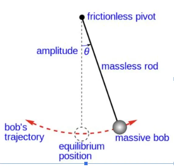
A simple pendulum is defined to have an object that has a small mass, also known as the pendulum bob, which is suspended from a light wire or string, such as shown in the figure below.

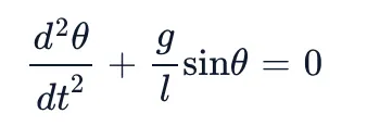
The dynamic behaviour of pendulum bob is important to understand the motion of simple pendulum. When the pendulum bob is given an initial push while it is at rest, it experiences a force sideways. It is displaced from its equilibrium position and starts to oscillate about the pivot point swinging back and forth. In general the motion of a simple pendulum is considered to be simple harmonic motion with constant amplitude and is given by the equation,

Error in movie M(ct) command

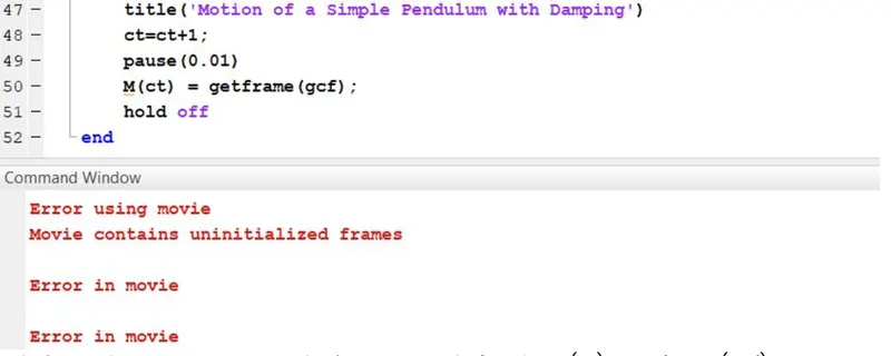
Solution – The counter ‘ct’ must be incremented after the M(ct) = getframe(gcf) command. If the counter is incremented before, then the movie will contain uninitialized frames.

video has been upload

https://youtu.be/Xc3EOs3tNPs

CONCLUSION:-

THEREFORE WE HAVE CREATED A MATLAB PROGRAM THAT HELPS TO COMPLETE ALL TASK GIVEN ABOVE