Project 2 - Rankine cycle Simulator

Aim:- Creation of Rankine cycle simulator from given input and reading the data from standard thermodynamic library of steam table.

• To create a Rankine Cycle simulator in MATLAB.
• To calculate the state point using function XSteam.
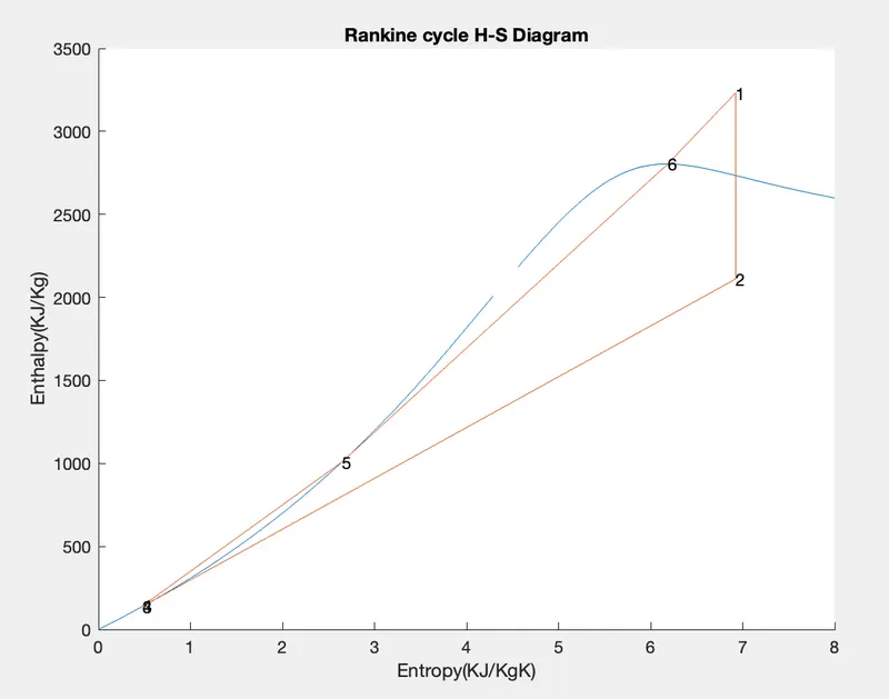
• To plot the T-S and H-S curve for given input in Rankine Cycle.
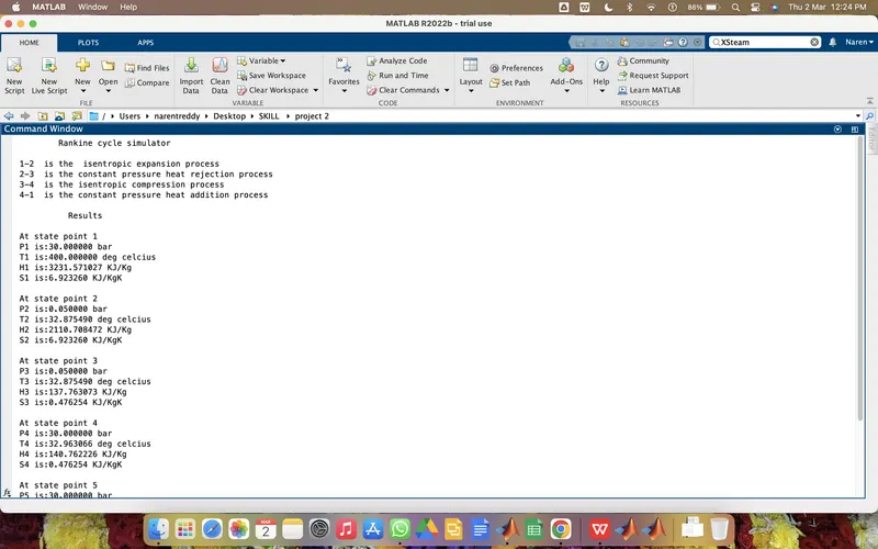
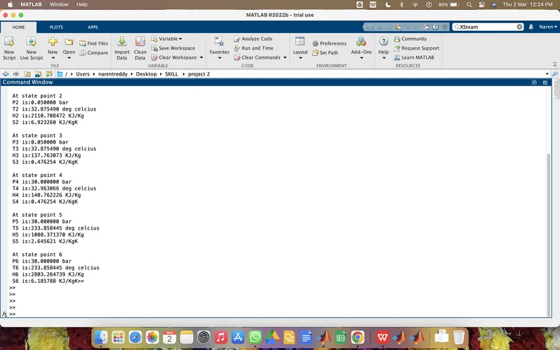
• To get output in the command window for each state point in cycle.

OBJECTIVES:- TO COMPLETE ALL TASK GIVEN ABOVE

PROGRAM:- CODING IN MATLAB

close all 
clear all
clc
% displaying rankine cycle simulator and its processess
disp("         Rankine cycle simulator")
fprintf('\n 1-2  is the  isentropic expansion process')
fprintf('\n 2-3  is the constant pressure heat rejection process')
fprintf('\n 3-4  is the isentropic compression process')
fprintf('\n 4-1  is the constant pressure heat addition process')
% variables for stage1 
p1 = 30;
t1 = 400;
h1 = XSteam('h_pT',30,400);
s1 = XSteam('s_ph',30,h1);
fprintf('\n\n           Results')
fprintf('\n\n At state point 1')
fprintf('\n P1 is:%f bar',p1)
fprintf('\n T1 is:%f deg celcius',t1)
fprintf('\n H1 is:%f KJ/Kg',h1)
fprintf('\n S1 is:%f KJ/KgK',s1)


% variables for stage2 
p2 = 0.05;
s2 = s1;
t2 = XSteam('T_ps',0.05,6.1858);
sf2 = XSteam('sL_p',p2);
sg2 = XSteam('sV_p',p2);
hf2 = XSteam('hL_p',p2);
hg2 = XSteam('hV_p',p2);
x = ((s2 - sf2)/(sg2 - sf2));
h2 = hf2 + (x*(hg2 - hf2));
v2 = XSteam('v_ph',p2,h2);
fprintf('\n\n At state point 2')
fprintf('\n P2 is:%f bar',p2)
fprintf('\n T2 is:%f deg celcius',t2)
fprintf('\n H2 is:%f KJ/Kg',h2)
fprintf('\n S2 is:%f KJ/KgK',s2)

% variables for stage3
t3 = t2;
p3 = p2;
s3 = XSteam('sL_p',p3);
h3 = XSteam('hL_T',32.875);
v3 = XSteam('v_ph',p3,h3);
fprintf('\n\n At state point 3')
fprintf('\n P3 is:%f bar',p3)
fprintf('\n T3 is:%f deg celcius',t3)
fprintf('\n H3 is:%f KJ/Kg',h3)
fprintf('\n S3 is:%f KJ/KgK',s3)

% variables for stage4
s4 = s3;
v4 = v3;
p4 = p1;
h4 = XSteam('h_ps',p4,s4);
t4 = XSteam('T_hs',h4,s4);
fprintf('\n\n At state point 4')
fprintf('\n P4 is:%f bar',p4)
fprintf('\n T4 is:%f deg celcius',t4)
fprintf('\n H4 is:%f KJ/Kg',h4)
fprintf('\n S4 is:%f KJ/KgK',s4)


% variables for stage6
p5 = p4;
t5 = XSteam('Tsat_p',p5);
h5 = XSteam('hL_T',t5);
s5 = XSteam('sL_p',p5);
fprintf('\n\n At state point 5')
fprintf('\n P5 is:%f bar',p5)
fprintf('\n T5 is:%f deg celcius',t5)
fprintf('\n H5 is:%f KJ/Kg',h5)
fprintf('\n S5 is:%f KJ/KgK',s5)


% variables for stage6
t6 = t5;
p6 = XSteam('psat_T',t5);
s6 = XSteam('sV_T',t6);
h6 = XSteam('hV_T',t6);
fprintf('\n\n At state point 6')
fprintf('\n P6 is:%f bar',p6)
fprintf('\n T6 is:%f deg celcius',t6)
fprintf('\n H6 is:%f KJ/Kg',h6)
fprintf('\n S6 is:%f KJ/KgK',s6)

% loop to find variables on saturation lines
t = linspace(0,400,1000);
for i=1:length(t)
s_line1(i)=XSteam('sL_T',t(i));
end

for j=1:length(t)
s_line2(j)=XSteam('sV_T',t(j));
end
for i=1:length(t)
h_line1(i)=XSteam('hL_T',t(i));
end

for j=1:length(t)
h_line2(j)=XSteam('hV_T',t(j));
end

% net work output calculation
w_turbine = h1 - h2;                          % work done by turbine
w_pump = h4 - h3;                             % work taken by pump
work = w_turbine - w_pump;                    % net work output
q_in = h1 - h4;                               % heat addition
q_out = h2 -h3;                               % heat rejection

% thermal efficiency
n = work/q_in;

%Back work ratio
BWR = w_pump/w_turbine;

% Specific steam consumption
ssc = 3600/work;

%plotting T-s graph
figure(1)
hold on
plot([s_line1 s_line2],[t t])
plot([s1 s2 s3 s4 s5 s6 s1],[t1 t2 t3 t4 t5 t6 t1])
text(s1,t1,'1')
text(s2,t2,'2')
text(s3,t3,'3')
text(s4,t4,'4')
text(s5,t5,'5')
text(s6,t6,'6')
title("Rankine cycle T-S Diagram")
xlabel('Entropy(KJ/KgK)')
ylabel('Temperature(K)')
axis([0,8,0,450])
%plotting h-s graph
figure(2)
hold on
plot([s_line1 s_line2],[h_line1 h_line2])
plot([s1 s2 s3 s4 s5 s6 s1],[h1 h2 h3 h4 h5 h6 h1])
text(s1,h1,'1')
text(s2,h2,'2')
text(s3,h3,'3')
text(s4,h4,'4')
text(s5,h5,'5')
text(s6,h6,'6')
title("Rankine cycle H-S Diagram")
xlabel('Entropy(KJ/KgK)')
ylabel('Enthalpy(KJ/Kg)')
axis([0,8,0,3500])

RESULTS :

FIGURE 1

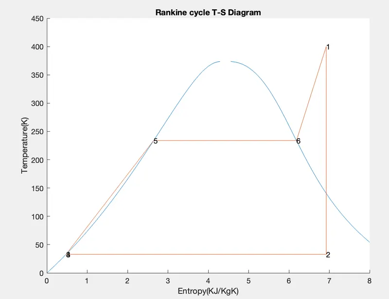
FIGURE 2

RESULTS IN COMMAND WINDOW

COMMANDS USED

• CLOSES ALL :- closes all figures whose handles are visible.
• CLEAR ALL: - clear removes all variables from the current workspace, releasing them from system memory
• CLC :- clc clears all the text from the Command Window, resulting in a clear screen.
• ( : ) colon operator to create regularly spaced vectors, index into arrays, and define the bounds of a for loop.]
• ( ; ) Suppress output display
• ( % ) Description Comment
• Plot :- Create a simple line plot and label the axes. Customize the appearance of plotted lines by changing the line color, the line style, and adding markers.
• Axis Labels : - Add axis labels to the chart by using the xlabel and ylabel functions.
• Add Title :-Add a title to the chart by using the title function. To display the Greek symbol π, use the TeX markup, \pi.
• FUNCTIONS:-Programs that accept inputs and return outputs. Both scripts and functions allow you to reuse sequences of commands by storing them in program files. Functions provide more flexibility, primarily because you can pass input values and return output values.
• fprintf all the molecular weights of the species. and then close the txt file using fclose command.
• strfind command to find before and after numbers of the coefficients then we will find remaining 14 coefficients and convert them to numbers from strings.

CONCLUSION:-

THEREFORE WE HAVE CREATED A MATLAB PROGRAM THAT HELPS TO COMPLETE ALL TASK GIVEN ABOVE