Week 4.1 - Solving second order ODEs
> AIM; SOLVING SECOND ORDER DIFFERENTIAL EQUATION FOR PENDULAM.
> PROBLEM STATEMENT;
In Engineering, ODE is used to describe the transient behavior of a system. A simple example is a pendulum
The way the pendulum moves depends on the Newtons second law. When this law is written down, we get a second order Ordinary Differential Equation that describes the position of the "ball" w.r.t time.
Similarly, there are hundreds of ODEs that describe key phenomena and if you have the ability to solve these equations then you will be able to simulate any of theses systems.
Your objective is to write a program that solves the following ODE. This ODE represents the equation of motion of a simple pendulum with damping
In the above equation,
g = gravity in m/s2,
L = length of the pendulum in m,
m = mass of the ball in kg,
b=damping coefficient.
Write a program in Matlab\Octave that will simulate the pendulum motion, just like the one shown in the start of this challenge.
use,
L=1 metre,
m=1 kg,
b=0.05.
g=9.81 m/s2.
Simulate the motion between 0-20 sec, for angular displacement=0,angular velocity=3 rad/sec at time t=0.
> SECOND ORDER DIFFERENTIAL EQUATION;
In mathematics, a differential equation is an equation that relates one or more unknown functions and their derivatives.[1] In applications, the functions generally represent physical quantities, the derivatives represent their rates of change, and the differential equation defines a relationship between the two. Such relations are common; therefore, differential equations play a prominent role in many disciplines including engineering, physics, economics, and biology.
Mainly the study of differential equations consists of the study of their solutions (the set of functions that satisfy each equation), and of the properties of their solutions. Only the simplest differential equations are solvable by explicit formulas; however, many properties of solutions of a given differential equation may be determined without computing them exactly.
> TYPES OF DIFFERENTIAL EQUATION;
Differential equations can be divided into several types. Apart from describing the properties of the equation itself, these classes of differential equations can help inform the choice of approach to a solution. Commonly used distinctions include whether the equation is ordinary or partial, linear or non-linear, and homogeneous or heterogeneous. This list is far from exhaustive; there are many other properties and subclasses of differential equations which can be very useful in specific contexts.
Ordinary differential equations[edit]
An ordinary differential equation (ODE) is an equation containing an unknown function of one real or complex variable x, its derivatives, and some given functions of x. The unknown function is generally represented by a variable (often denoted y), which, therefore, depends on x. Thus x is often called the independent variable of the equation. The term "ordinary" is used in contrast with the term partial differential equation, which may be with respect to more than one independent variable.
Linear differential equations are the differential equations that are linear in the unknown function and its derivatives. Their theory is well developed, and in many cases one may express their solutions in terms of integrals.
Most ODEs that are encountered in physics are linear. Therefore, most special functions may be defined as solutions of linear differential equations (see Holonomic function).
As, in general, the solutions of a differential equation cannot be expressed by a closed-form expression, numerical methods are commonly used for solving differential equations on a computer.
Partial differential equations[edit]
A partial differential equation (PDE) is a differential equation that contains unknown multivariable functions and their partial derivatives. (This is in contrast to ordinary differential equations, which deal with functions of a single variable and their derivatives.) PDEs are used to formulate problems involving functions of several variables, and are either solved in closed form, or used to create a relevant computer model.
PDEs can be used to describe a wide variety of phenomena in nature such as sound, heat, electrostatics, electrodynamics, fluid flow, elasticity, or quantum mechanics. These seemingly distinct physical phenomena can be formalized similarly in terms of PDEs. Just as ordinary differential equations often model one-dimensional dynamical systems, partial differential equations often model multidimensional systems. Stochastic partial differential equations generalize partial differential equations for modeling randomness.
Non-linear differential equations[edit]
A non-linear differential equation is a differential equation that is not a linear equation in the unknown function and its derivatives (the linearity or non-linearity in the arguments of the function are not considered here). There are very few methods of solving nonlinear differential equations exactly; those that are known typically depend on the equation having particular symmetries. Nonlinear differential equations can exhibit very complicated behaviour over extended time intervals, characteristic of chaos. Even the fundamental questions of existence, uniqueness, and extendability of solutions for nonlinear differential equations, and well-posedness of initial and boundary value problems for nonlinear PDEs are hard problems and their resolution in special cases is considered to be a significant advance in the mathematical theory (cf. Navier–Stokes existence and smoothness). However, if the differential equation is a correctly formulated representation of a meaningful physical process, then one expects it to have a solution.[11]
Linear differential equations frequently appear as approximations to nonlinear equations. These approximations are only valid under restricted conditions. For example, the harmonic oscillator equation is an approximation to the nonlinear pendulum equation that is valid for small amplitude oscillations (see below).
> PROGRAM CODE;
> ODE equation;
clear all
close all
clc
% defining the geometric parameters for the pendulam.
b = 0.05;
g = 9.81;
l = 1;
m = 0.5;

% define the initial conditions for the displacement,velocity,and time.
theta_0 = [0;3];
t_span = linspace(0,20,100);
% ode45 is used to solve the highier order non stiff ordinary differential
% equations.
% ode 45 uses the range kutta fourth order method to perform the numerical
% integration at each point to the solution.
% '@' is used for the function handle.
% 'results' is the two column matrix which stores the displacement and
% velocity.
% @('t,theta') are the anonymous variables ,are the variables those are
% defined no where in the program.

[t,results] = ode45(@(t,theta) ode_func(t, theta, b,g,l,m),t_span ,theta_0);

% use figure command to make the single window for the program.

figure(1)
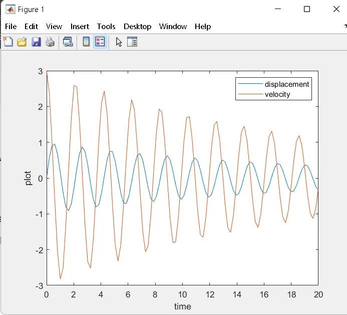
plot(t,results(:,1))
hold on
plot(t,results(:,2))
ylabel('plot')
xlabel('time')
legend('displacement','velocity')
THETA = results(:,1);
ct = 1;
for i = 1:length(THETA)

    position = THETA(i);

    figure(2)
    x0 = 0;
    y0 = 0;

    x1 = l*sin(position);
    y1 = -l*cos(position);

    plot([x0 x1],[y0 y1], 'linewidth',5)
    hold on
    plot(x1,y1,'.','markers',50)
    hold on
    plot([-5,5],[0,0],'linewidth',8)
    hold off
    axis([-9,9,-4,4])
    pause(0.05)
    M(ct) = getframe(gcf);
    ct = ct+1;
end
% create the movie animation.
movie(M)
videofile = VideoWriter('pendulam','Uncompressed AVI');
open(videofile)
writeVideo(videofile,M)
close(videofile)
CFEATE THE FUNCTION SCRIPT FOR THE ode_func.
function[dtheta_dt] = ode_func(t,theta,b,g,l,m)

theta1 = theta(1);
theta2 = theta(2);
dtheta1_dt = theta2;
dtheta2_dt = (-b/m)*theta2 - (g/l)*sin(theta1);
dtheta_dt = [dtheta1_dt;dtheta2_dt];

end
> COMMANDS USED IN THE ABOVE PROGRAM;
1) figure() ; this command is used Fix the figure window so that we can see all the plots those are of diffrent positions at a single figure window.
2) axis(); this command is used to set te minimum and maximum limits for the x and y axis, for setting the domain for the figure window.
3) videowriting in MATLAB;
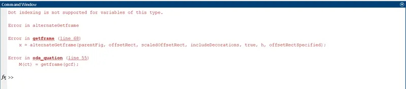
for creating the animation in the MATLAB we have to execute the statement "" M(ct) = getframe(gcf) "".
> counter_variable(ct); It helps in proper indexing in which the captured frames will be indexed sequentially.
> getframe(); it captures the figure as frames.
> To create the movie animation in the MATLAB;
movie(M); this command is used to plays the movie frames those are sequentially arranged in the array M.
VideoWriter(); This command will create a videofile of specified name and format,initially this is empty video file.
writeVideo(); THis command is used to write the frames those are sequentially arranged in the array 'M' in the videofile that is created by the command 'videowiter()'.
> Plot between the displacement and the time.
> Animation for the pendulam;
> errors;