Week 4.1: Project - Steady state simulation of flow over a throttle body

Aim -TO set up steady stae simulation fror a flow over a throttle body.

objectives-

1.Set up and run the steady state simulation for flow over throttle body.

2.Post process the results and to show pressure and velocity contours and to plot foir velocity and pressure.

Theroy-

Throttle boby is used to regulate the flow of petrol and air mixture required for combustion in the gasoline engines. The amount of combustion and the polluants depennds upon the position of the valve in the throttle body.generally the throttle valves are butterfly valves.

1.preprocessing - First import the cad stl file in to converge studio .For better flow we delete the outside covering of the elbow and at both inlet and at the outlet.

ii. Boundary condtion - After imorting geometry we next create bounadary condtion. The elbow is selected as the wall and the motion of the wall is given as stationery since the velocity is going to be zeo at the walls hence turblent kinetic engery is given as zero normal gradient and turblent disssipation as the wall motion.similary the same boundary condtion is given for the throttle.and For inlet the flow is inflow type and inlet pressure is given as 1e5 bar at temperature 300K. and at the outlet the flow is of outflow and outlet pressure is 1 bar .at the both inlet and at the outlet the air is selected as fluid mixture.

2.Solvers

i.Solvers and simulation time parametrs - as above project involves no moving part hence we solver as steady solver with full hydrodynamic.

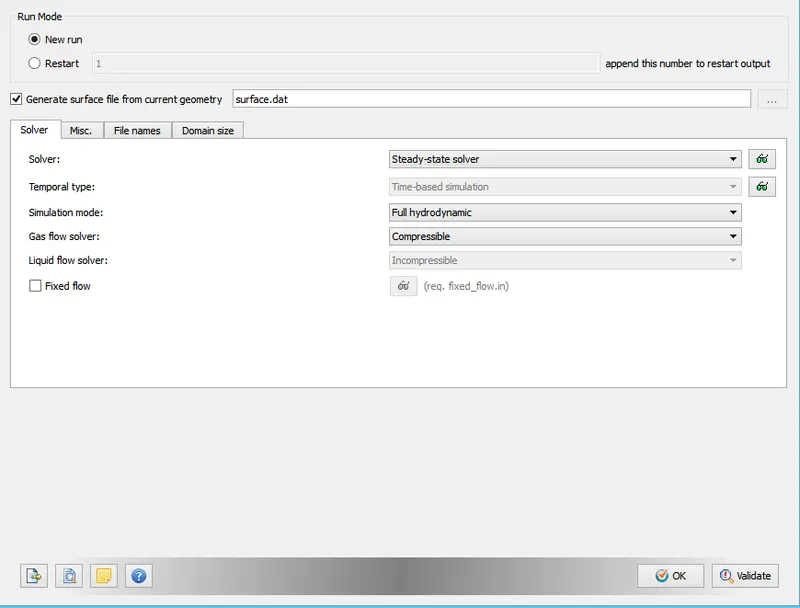
and time time parametrs is shown below in the table

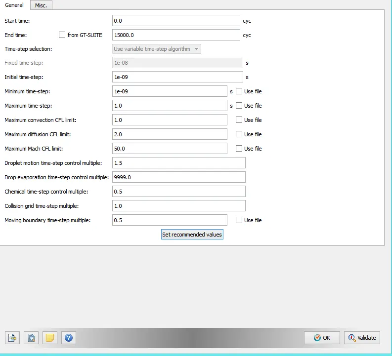
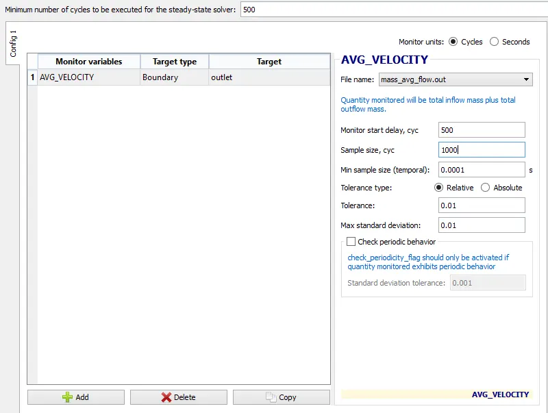
the simulation time starts from 0 cycles (here cycles for steady state and sec for transient solver)the end of the simulation depends on the solution attaing the convergence i.e the steady state starts monntoring for every cycles ande for every 1000 cycles it will check the tolerance of the average parameters for an example for 1000 cycles the average velocity is 2.25m/sec and for next 1000 cycles the average velocity is 2.24 and the tolerance bewteen the two cycles is 0.01 at this the simulation stops as it reached given tolerance if tolerance is not reched again its going to run but its going to run atleast minimum 500 cycles. and in the above plot the end time is taken apporixamately 15000 its not necessary for the simulation to run 15000 cycles.

3.Postprocessing

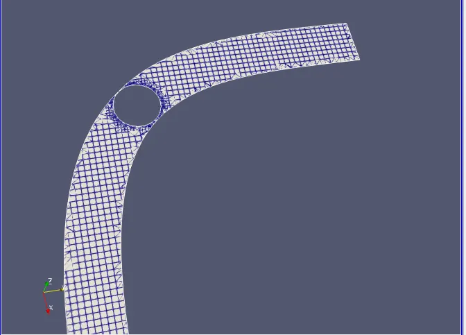
figure-mesh for steady state transient

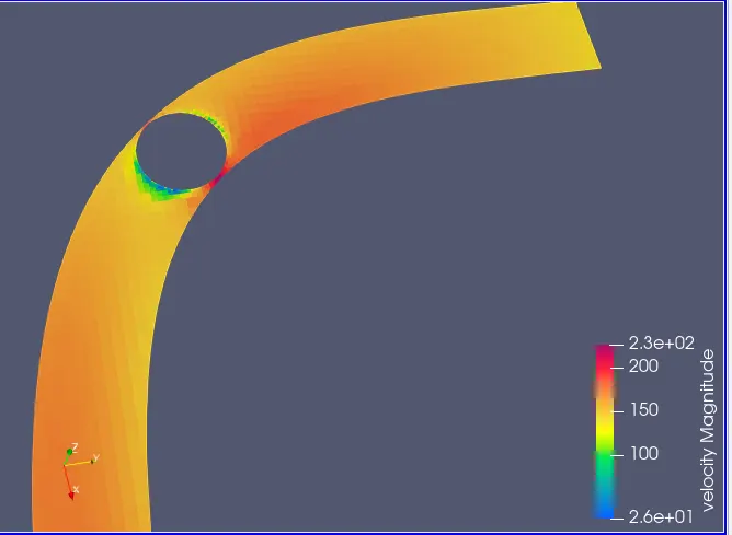
fig-velocity countour for steady state throotle

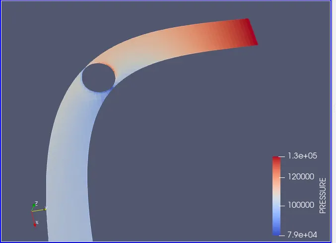
figure-pressure countour for steady state countour

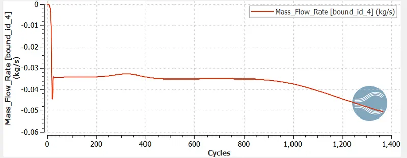figure- mass flow rate at the inlet

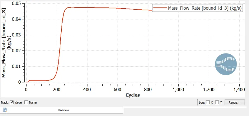
figure - mass flow rate at the outlet

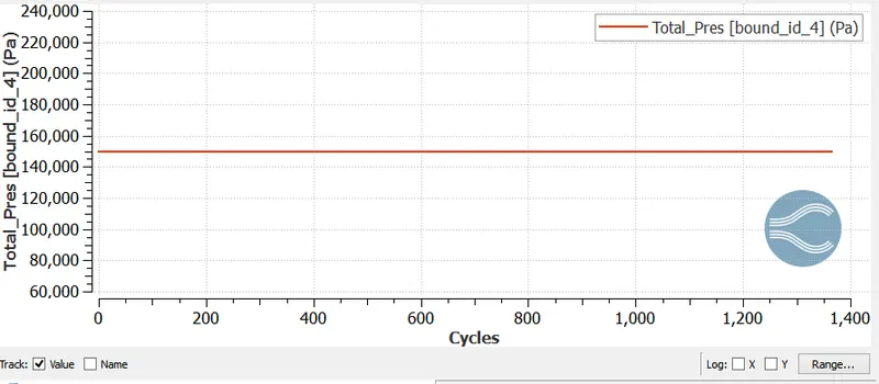
figure- Total pressure at inlet

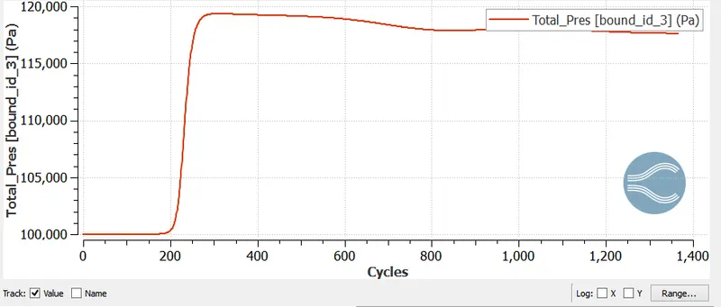
figure-Total pressure at the oulet

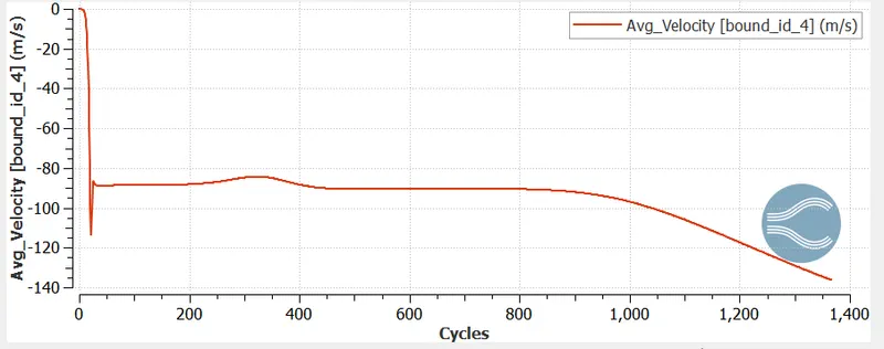
figure-Average-velocity at the inlet

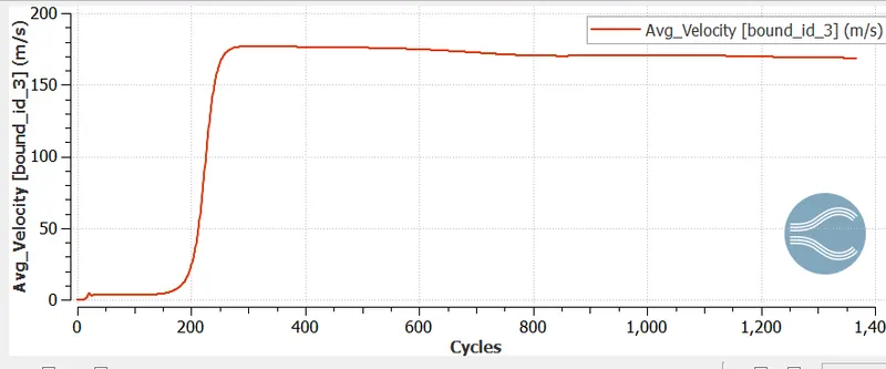
figure-Average velocity at the outlet

Conclusion-

as the cross section at inlet is more so pressure gradient(dp/dx)increases and velocity gradient (du/dy) decreases. and cross section varies near the throotle hence at the outlet since the small cross sectional area the pressure gradient decreases and the velocity gradient increases.as near the throotle the cross section decreases the pressure gradient decreases and the velocity increases.

sa

sa