Week 4.1: Project Steady state simulation of flow over a throttle body

Objective:

Steady state simulation of flow over a throttle body.

Introduction:

A throttle is a mechanism by which flow is managed by constrction. Examples of throttling process are flow through a partially openned valve, flow through a very small opening or a flow through a porous plug.

• Characteristics of throttling :

Throttling is an irreversible process and an isenthalpic process.

In fuel injected engines, the throttle body is a part of the air intake system , that controls the amount of air entering the system. The largest piece inside the throttle body is the throtle plate, a butterfly valve regulates the air flow.

Geometry:

The stl file of the elbow is imported into converge studio.

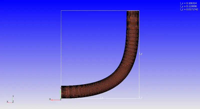
This is a elbow, the throttle body is situated inside the elbow walls.

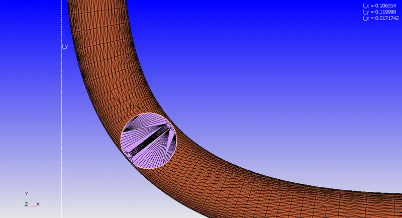
The geometry had many open edges initially. Using the patch tool , the geometry is repaired.

Boundary conditions:

To flag the boundaries namely into the following parts - inlet,outlet,throttle body,elbow walls.

The Throttle body in this particu;ar case is basically a surface and can be selected using the suraface selection option.

Finally the diagnosis tool is used and the oriebntation of the normals are checked.

Case set up:

The simulation environment of converge studio includes:

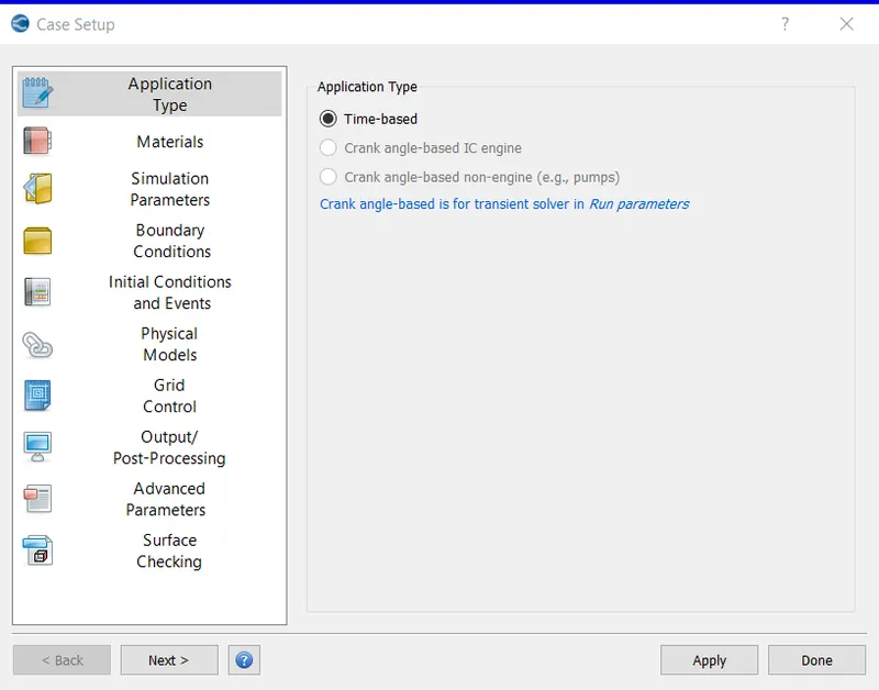
• Application type:

This simulation is essentially a time based application.

• materials:

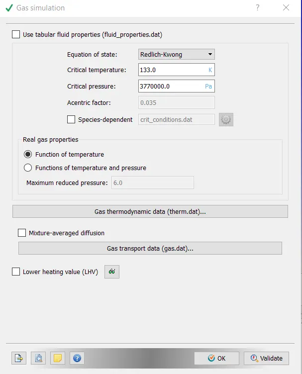
Predefined mixture is selected as air. gas simulation is checked. Species checkbox is checked. The species are O2 and N2.

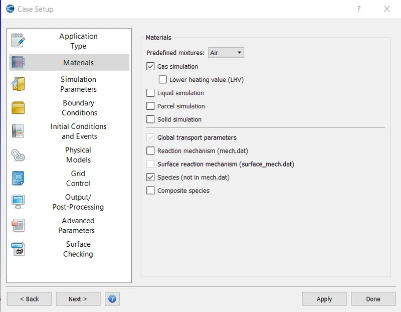
The gas simulation box is kept unchanged and the default values loaded by converge studio is worked upon with.

Global parameters:

Turbulent Prandtl number	0.9
Turbulent schmidt number	0.78

• Simulation parameters:

Solver	Steady state solver
Simulation mode	Full-hydrodynamic
Gas flow solver	Compressible

The mass flow rate is selected as the steady state monitor , with boundary as the target type . The steady state monitor variable actually gets monitored through out the simulation.

The monitor start delay is 10,000 cycles and the sample size is 1000 cycles. This means the monitor variable will start getting monitored ater 10000 cyles.

Simulation time parameters:

start time	0
end time	15000 cycles
initial time step	1e-9
minimum time step	1e-9
maximum CFL convection limit	1

Solver parameters:

Navier stokes solver scheme	PISO
NAvier stokes solver	density based solver

• Boundary Conditions:

1) Elbow walls :

Boundary type is wall. since it is fixed and acts as wall.

Velocity boundary conditions - The wall motion type is stationary and the surface movement is set to fixed.

Temperature boundary conditions is set to zero normal gradient .

The turbulent kinetic energy boundary condition is Specified value (DI).

2) Inlet :

Boundary type is Inflow.

Pressure boundary condition - Total pressure is checked and the value is 1.5e5 pascals. The condition is specified value(DI)

Temperature boundary condition - Specified valkue(DI)

Species boundary condition- specified value(DI) , Air (O2 and N2) is selected.

3) Outlet:

Boundary type is Outflow.

The pressure boudary condition is specified value (DI) with pressure = 100000 pa.

The velocity boundary condition is zero normal gradient. The backflow temperature is 300K . The species backflow is selected as Air(O2 and N2).

4)Throttle body:

Boundary type is wall

Velocity boundary conditions-

Wall motion type is stationary and the surface movement is fixed. No slip condition is enabled.

Temperature boundary conditions- zero normal gradient

Turbulent kinetic energy boundary conditions - Zero normal gradient.

• Region initialization:

Temperature	300 K
Pressure	101325 Pa
Species	Air(O2,N2)
Region name	Region0

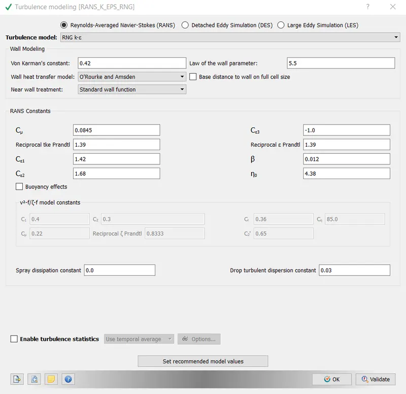
• Turbulence modelling:

RNG k-epsilon turbulence model is selected. Other parameters are left as it is.

• Grid sizing:

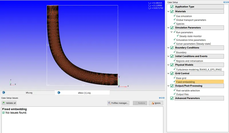
Base grid size :

dx=0.003 meters ;dy=0.003 meters;dz=0.003 meters.

Embedding:

The boundry embedded is Throttle . Permanent embedment is done. Scale=3 and amebdded layers =2.

This concludes the Case set up.

Simulation:

The command prompt is opened. The mpi execuatble file is and the converge.exe file is imported into the folder in which the input files are kept.

By the command mpiexec.exe -n 4 converge.exe restricted , the simulation is ran

Four processors are used in the simulation.

After the simulation is complete, the output files are converted into inline binary atk format for post processing in PARAVIEW. PARAVIEW is an open end post processing software.

Post processing:

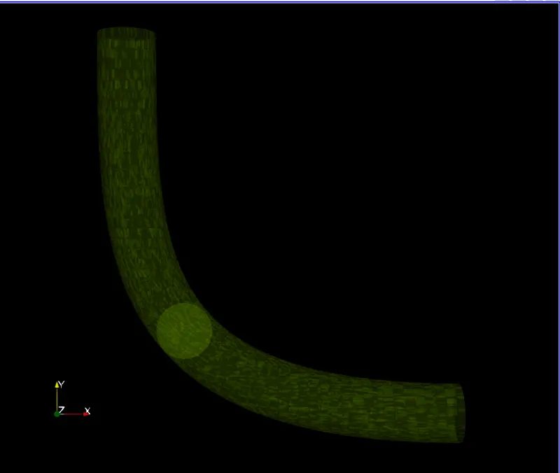
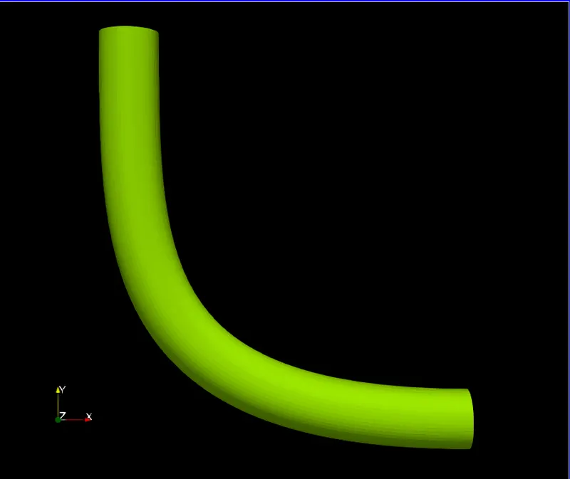
The first image shows the throttle body inside the elbow wall. This is done by changing the opacity of the elbow wall.

A slice is cut out with the normal direction of the slice along the z direction.

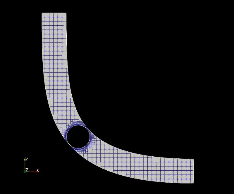
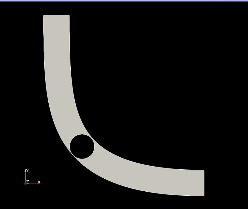
The surface with edges command shows the generated grid .

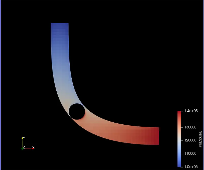
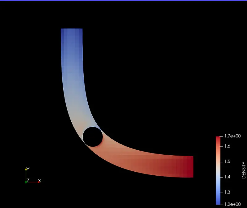
By coloring with the pressure, velocity and density , the different contours are obtained.

Velocity contour:

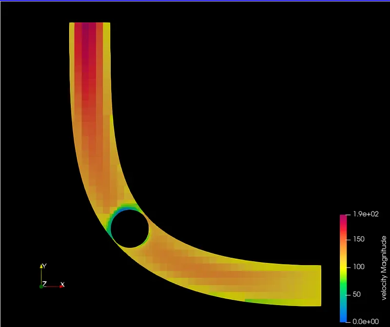
There is a zone where the velocity of the fluid gets to zero around the throttle body.

Pressure contour:

3) Density contour:

A glymph is created with the velocity array:

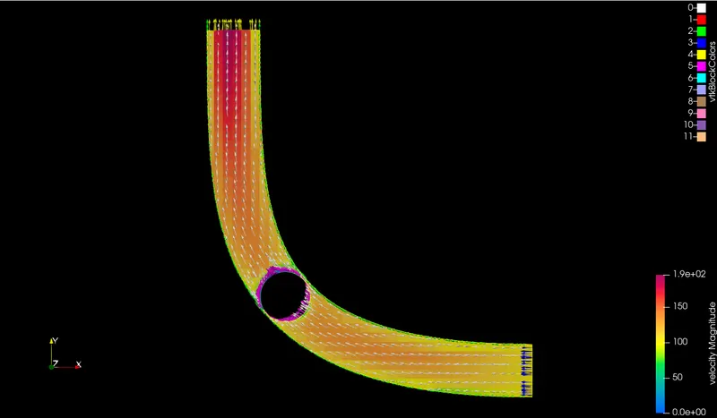
The arrow shows the direction of the flow inside the elbow. The arrow signifies the velocity vector.

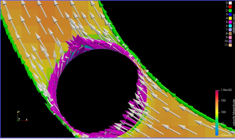
The zoomed in section of the throtte body. There is a flow along the sides , since the throttle valve is not perfectly sealing the geometry.

Since the valve is open, there is no serious pressure drop across the valve.

plots:

1) Average velocity at inlet and outlet:

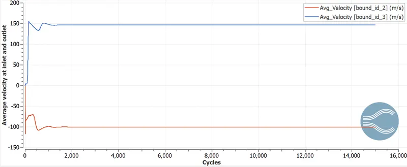
the solution converges actually at the 1000 cycles.

2) Static pressure at inlet and outlet:

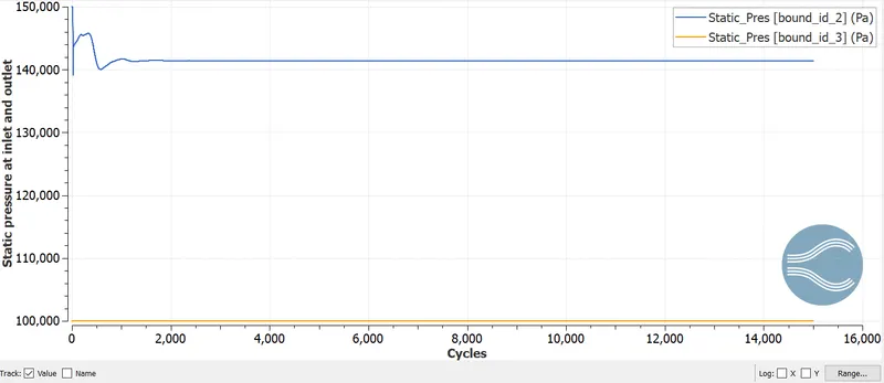
The static pressure at the inlet attains at steady state value of something around 140000pa at nearly 1000 cycles. At the outlet the static pressure is 100000 pa.

3) Total pressure at inlet and outlet:

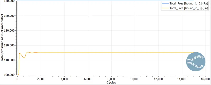
the total presssure at the inlet is constant at 150000 Pa. At the outlet it attains a steady state value of 115000 Pa at nearly 1200 cycles.

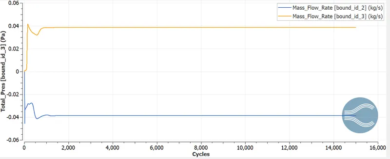
4) Mass flow rate at inlet and outlet:

5) Total cell count:

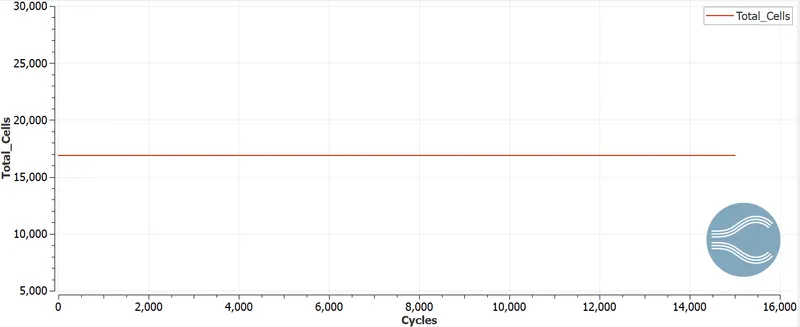
The total cell counts is 17000. It is equally distributed among the four processors. rank0,rank1,rank2,rank3. For better accuracy, the grid might be made bit finer.

The animation file is uploaded as https://youtu.be/ltuYohFmWI0

Conclusion:

A steady state simulation of flow about a throttle body is performed. With the increase in the number of cells by dcreasing the grid size further, more accurate results can be obtained. Along the wall of the throttle body, there is zero velocity due to the no slip condition.