Throttle body Steady-State simulation using Converge.

Aim: Steady-state simulation of flow over a throttle body

Objective:

• Set up and run the steady-state simulation for flow over the throttle body.
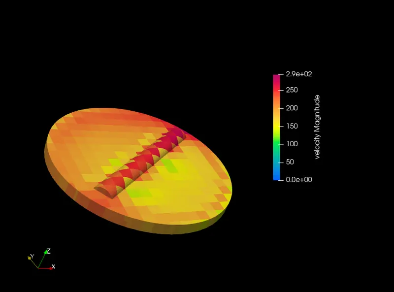
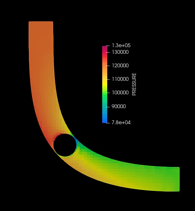
• Post-process the results and show pressure and velocity contours.
• Show the mesh (i.e surface with edges)
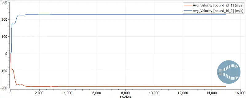
• Show the plots for pressure, velocity, mass flow rate, and total cell count.
• Create an animation in which its throttle movement should be visible.

Introduction

Throttle

A throttle is a mechanism by which the fluid flow is managed by construction or obstruction. An engine's power can be increased or decreased by the restriction of inlet air due to the presence of a throttle. The term throttle can be used to increase the efficiency of the car, the car accelerator pedal can be used as a throttle to increase the efficiency of the engine. It is used as a throttle in the field of aviation, known as a thrust lever in jet engine-powered aircraft. For steam locomotive, the valve which controls the regulation of gas is called a regulator.

Application of throttle

The throttle is a mechanism that is used to increase or decrease the power of the engine by restricting the flow of inlet gases coming through it. There are numerous applications of the throttle mechanism which are listed below

• Internal Combustion Engines
• Fuel Injected Engines
• Reciprocating Engine Aircraft
• Steam locomotives
• Automobiles

Case-setup

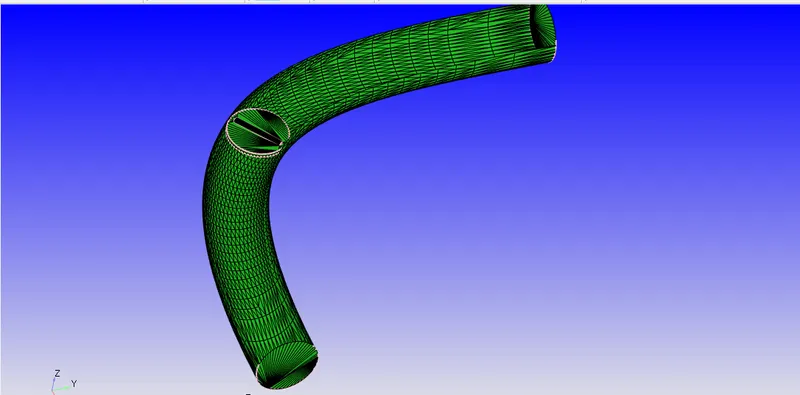
The internal flow simulation does not involve the usage of the external boundary, the external boundary is of special interest when there is a CHT simulation setup. The external boundary can be deleted by selecting the triangle option from the ribbon and then hitting the "D" button on the keyboard by enabling the hotkeys. The other alternative is selecting the "Repair" option from the "Geometry Dock" window and selecting the entity and hitting "Apply".

The diagnosis dock is selected from the "View" option and the "Find" option is selected. It is found that there are 211 open edges in the geometry ("Intersections(0)","Nonmanifold Problems(0)","Open Edges(211)", "Overlapping Tris(0)","Normal Orientation(0)","Isolated tris (0)".

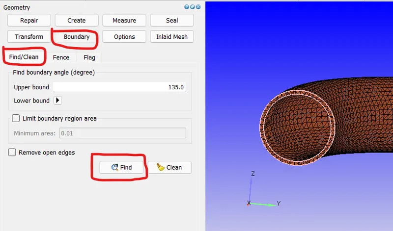
To remove open edges from the geometry, the "Repair" option in the "Geometry Dock" is selected, under "Patch" the "Open Edges" are selected viz (inlet and outlet) of the geometry, and then "Boundary Flagging" is done to make "Open Edges" in the resulting geometry to "0".

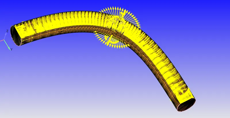
The "Normal Toggle" is selected from the ribbon, upon selecting the normal toggle it was observed that the normal is pointing outside the volume, technically the normal should point inside the volume where the fluid is flowing. Therefore in the geometry dock, the "Transform" option is clicked. The "Normal" tab is selected from the geometry dock and one of the triangles containing the normal pointing outward is selected. The "Apply" option is selected for removing the normals.

The "Case Setup Dock" is selected from the "View" and "Begin Case Setup" is executed.

The "Time" based "Application" type is selected. The "Material" is selected and the predefined mixture is selected as air. The "Reactant mechanism" is checked off because it is not a combustion problem. The species is selected and the "Apply" is clicked.

Under "Gas simulation" the Equation of state is selected as "Redlich Kwong", the critical temperature is 133K and the critical pressure is 3770000Pa.

The Turbulent Prandtl number is 0.9 and the Turbulent Schmidt number is 0.78 under Global Transport parameters.

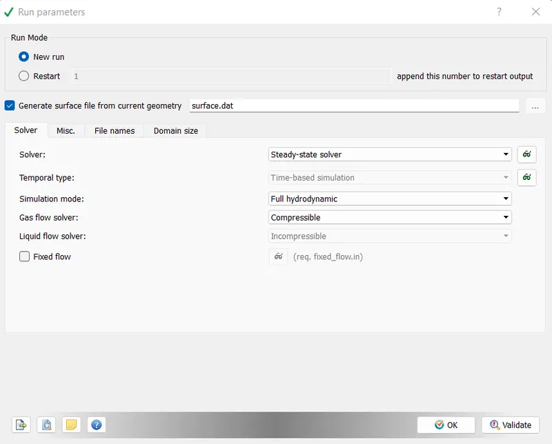
The O2">O2 and the N2">N2 are selected as species. Under "Run parameters" the "Steady-state solver" is selected. The "Temporal type" is locked for the steady-state. The "simulation mode" is selected as "Full Hydrodynamic" because the geometry is simple so while creating the mesh inside the geometry it solves the NS equation as well, but if the geometry is complex "No hydrodynamic solver" is selected as such if there is an error it will point out immediately while creating the mesh, otherwise if the hydrodynamic solver is selected then it will be very tedious to identify the error in the simulation case set up.

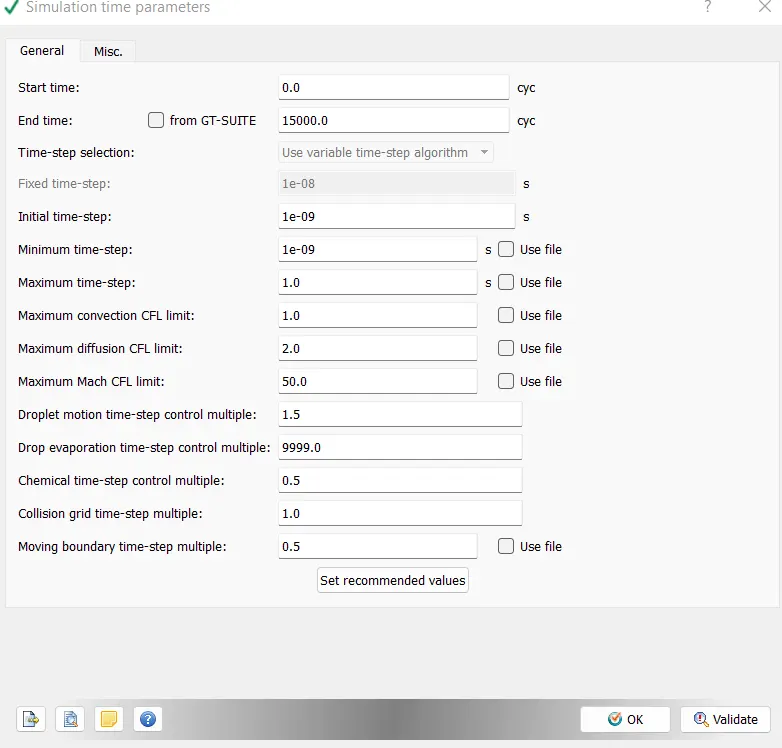
Under "Simulation time parameters" end time is chosen as 15000 cycles (steady-state). The initial and minimum time step is 1e-09 s. The maximum time step is 2s, and the maximum convection CFL limit is 1 and the rest are default values.

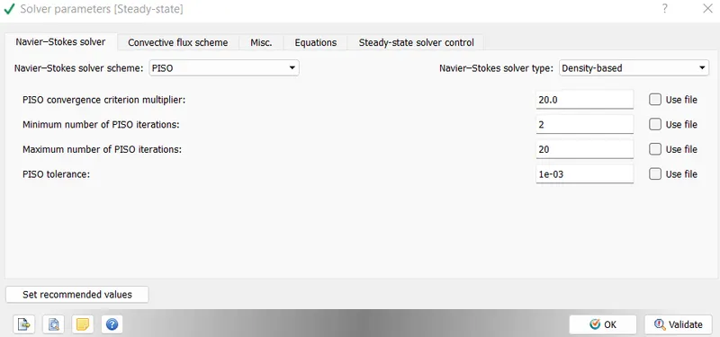
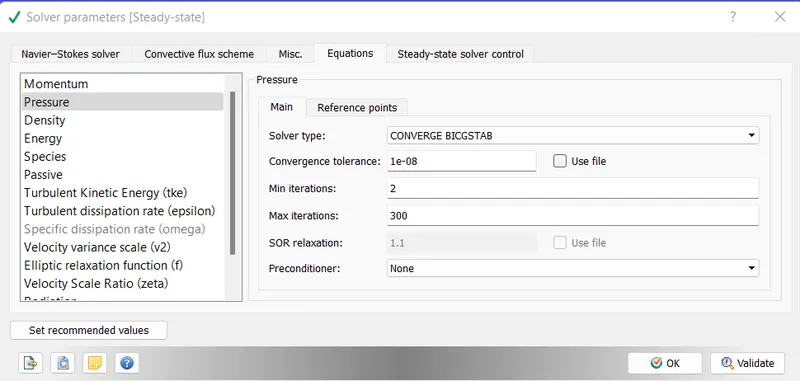
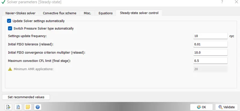
The "Pressure" "Equation" is selected under the "Solver parameter" and the "Preconditioner" is selected to "None". The "Maximum convection CFL limit (final stage)" is set to 0.5.

Regions and Initialization

In the "Region and Initialization" the mass fraction of O2">O2 and N2">N2 were created and named "Region 0" and the same is updated in the boundary condition region name. These are the initial condition and will be washed out after the solution has converged.

Steady-State Monitor

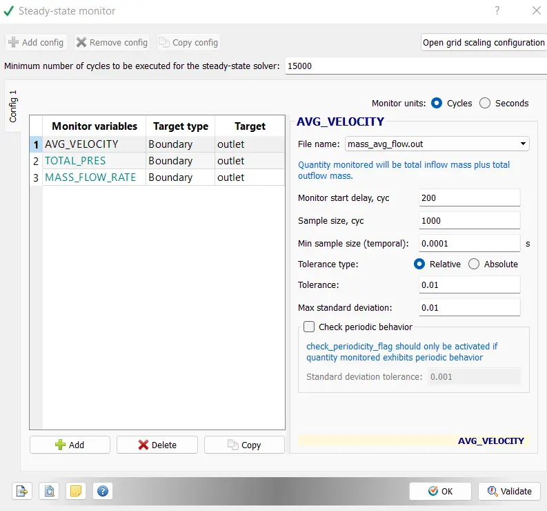
The monitor variables are added in the "Steady-state monitor". Avg Velocity, Mass flow rate, and Total Pressure have been added and the target area is selected as output. The minimum number of cycles to be executed for the steady-state solver is 15000 which signifies that the solver will run for a minimum of 15000 cycles if the solution reaches a convergence value before 15000, then the simulation will stop at 15000, but if the solution reaches a convergence value after 15000 then it will terminate at that moment. The solver checks the difference in the value of two consecutive sample sizes (1000) and matches it with the tolerance value to stop the solution. The converge-CFD software saves a lot of time and computational energy by tracking the solution when it reaches a steady state.

Setting up of Turbulence model

The Realisable k-ε">k-ε model is selected from the case-setup tree for the above-said simulation. Since the size of the eddies is restricted near the wall and the maximum size of the eddies is formed away from the wall. It is well suitable for resolving flows in the logarithmic flow region where y+ ranges from 30 to 300 and flow involving a high Reynolds number.

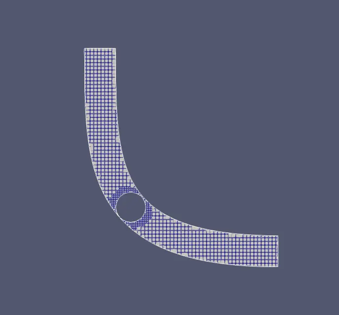
Mesh-0

Base-grid-size : 2e-3m

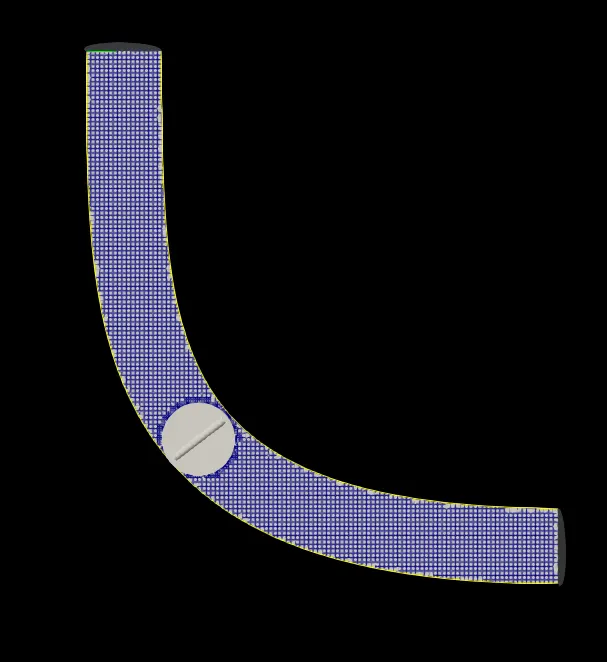
The mesh is coarse, and it involves the application of fixed embedding.

mesh 2

Line plots

Velocity

Pressure

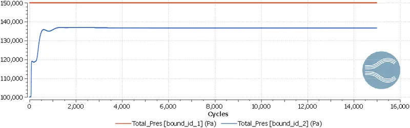
Mass flow rate

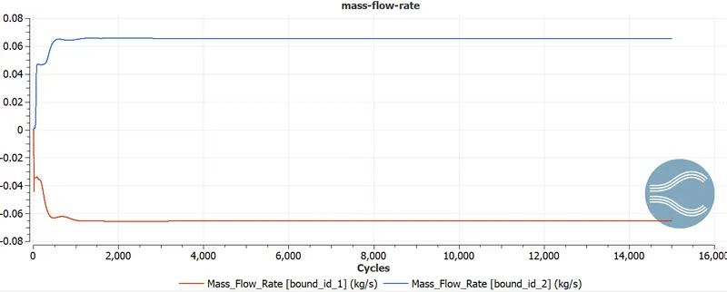
Total cell count

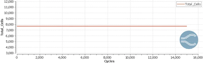
Contour plots

Velocity

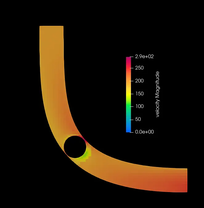
Pressure

Animation for mesh1

Velocity

Pressure

streamlines

Conclusion

• The steady-state simulation of flow over a throttle body was carried out successfully by the "Converge-CFD" software and the "Cygwin" command terminal.
• The Realizable k-epsilon model was used for modeling the turbulent flow in the pipe. The eddy movement created by the turbulent flow near the wall is less in size whereas as we move away from the wall of the pipe the size of the eddy grows considerably. The turbulent flow is characterized by unsteady velocity fluctuations and highly disordered motions as seen from the streamlines.