Week 4.1 - Genetic Algorithm

GENETIC ALGORITHM

MAIN PROGRAM

clear all
close all
clc


%% defining our search space
x = linspace(0,0.6,150);
y = linspace(0,0.6,150);

%% evaluating stalagmite fuction

for i = 1:length(x)
    for j = 1:length(y)
    inputs(1)=x(i);
    inputs(2)=y(j);
    f(i,j)=stalagmite(inputs);
    end
end

%% generate surface of the plot
num_cases=50;

%% stalagmite without bound case 
tic
for k= 1:num_cases
    [inputs,fopt(k)]=ga(@stalagmite,2);
    xopt(k)=inputs(1);
    yopt(k)=inputs(2);
end

figure(1)
subplot(2,1,1);
surfc(x,y,-f);
shading interp
hold on
plot3(xopt,yopt,-fopt,'Marker','o','MarkerSize',6,'MarkerFaceColor','r');
title('unbounded inputs')
xlabel('x value');
ylabel('y value');
grid on
subplot(2,1,2)
plot(fopt)
xlabel('iterations')
ylabel('function maximum')
study_1=toc;



%% study2 statistical behaviour with upper and lower bounds
tic

for k = 1:num_cases
    [inputs,fopt(k)]=ga(@stalagmite,2,[],[],[],[],[0;0],[0.4,0.4]);
    xopt(k)=inputs(1);
    yopt(k)=inputs(2);
end

figure(2)
subplot(2,1,1);
surfc(x,y,-f);
shading interp
hold on
plot3(xopt,yopt,-fopt,'Marker','o','MarkerSize',6,'MarkerFaceColor','r')
title('upper and lower bounds')
xlabel('x value');
ylabel('y value');
grid on
subplot(2,1,2)
plot(fopt)
xlabel('iterations')
ylabel('function maximum')
study_2 = toc;

tic


%% study 3 incresing Ga iteration
options=optimoptions('ga');
options=optimoptions(options,'PopulationSize',270);

tic

for k = 1:num_cases
    [inputs,fopt(k)]=ga(@stalagmite,2,[],[],[],[],[0;0],[0.4,0.4],[],options);
    xopt(k)=inputs(1);
    yopt(k)=inputs(2);
end
figure(3)
subplot(2,1,1);
surfc(x,y,-f);
shading interp
hold on
plot3(xopt,yopt,-fopt,'Marker','o','MarkerSize',3,'MarkerFaceColor','r')
title('increase in population')
xlabel('x value');
ylabel('y value');
subplot(2,1,2)
plot(fopt)
xlabel('iterations')
ylabel('function maximum')
study_3 =toc;

FUNCTION PROGRAM

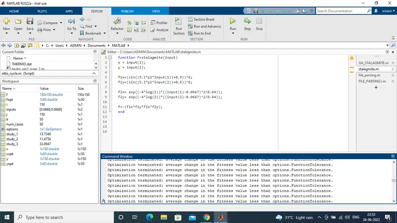
function f=stalagmite(input)
x = input(1);
y = input(2);

f1x=(sin((5.1*pi*input(1))+0.5))^6;
f1y=(sin((5.1*pi*input(2))+0.5))^6;

f2x= exp((-4*log(2))*((input(1)-0.0667)^2/0.64));
f2y= exp((-4*log(2))*((input(2)-0.0667)^2/0.64));

f=-(f1x*f1y*f2x*f2y);
end

 OUTPUT PLOTS FOR 3 STUDIES

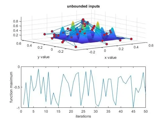
 UNBOUND

 

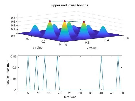
UPPER BOUNDS

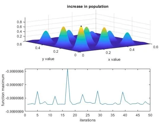
POPULATION GROWTH

EXPLAINATION ABOUT THE PROGRAM

• First step defining our search space x and y values are given to the inputs using the linspace command to spilted the values 
• next stage evaluating the stalagmite function using for loop
• two vectors using this stage i , j because two for loop usiing 
• in the program process we need 50 number of cases
• and mention time using time command tic

     study 1

• go to the first study simple fuctions without any bounds the input vector is k and using the for loop to run the stalagmite function
• in this stage genetic algorith GA is running in the for loop
• GA genetic algorithm is nothing but constrained and unconstrained optimization problem based on a natural selection process
• in this stage use the genetic algorith tool box we found the stalagmite function 
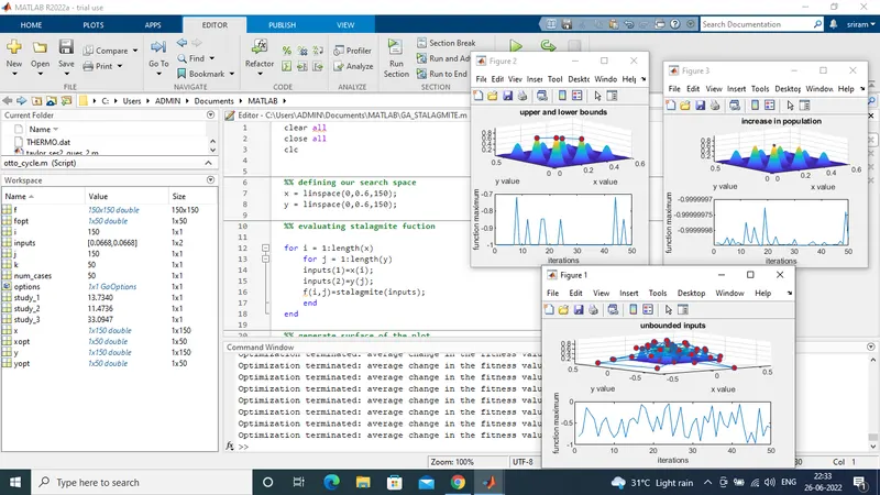
• output for the first study is denoted by figure 1 
• in the out put stage we using common commands like subplot,surfc,shading,hold on,plot3,xlabel ,ylabel and title 
• this output showed in above image 

     study 2

• in case study 2 we find theupper and lower bounds 
• in this stage also we using for loop
• in the stage one what can we do at the same think follow by the stage 2 but function only differ 
• extra some null matrix add to the GA function
• after end the loop we find the output 
• output is denoted by figure 2
• subplot values are 2,1,1 and using some comman commands to find the output
• study 2 result mentioned in above

     study 3

• study 3 is optimization of the maximum population 
• in the stage we use the optimoptions tool in GA
• we found the options value
• and next stage using the for loop to find the population 
• using bu ga stalagmite function
• here after same by the 1st and 2 nd stage we found the output in plot command denoted by figure 3
• the maximum population mentined in above results 

SCREEN SHOT ABOUT MAIN PROGRAM

SCREEN SHOT ABOUT FUNCTION PROGRAM