Week 4.1 - Genetic Algorithm

1. The algorithm begins by creating a random initial population.

2. The algorithm then creates a sequence of new populations. At each step, the algorithm uses the individuals in the current generation to create the next population. To create the new population, the algorithm performs the following steps:

   • Scores each member of the current population by computing its fitness value. These values are called the raw fitness scores.

   • Scales the raw fitness scores to convert them into a more usable range of values. These scaled values are called expectation values.

   • Selects members, called parents, based on their expectation.

   • Some of the individuals in the current population that have lower fitness are chosen as elite. These elite individuals are passed to the next population.

   • Produces children from the parents. Children are produced either by making random changes to a single parent—mutation—or by combining the vector entries of a pair of parents—crossover.

   • Replaces the current population with the children to form the next generation.

3. The algorithm stops when one of the stopping criteria is met.
4. The algorithm takes modified steps for linear and integer constraints.
5. The algorithm is further modified for nonlinear constraints.

Advantages of Genetic Algorithm,

• The concept is easy to understand.
• It has excellent parallel capabilities.
• GA use probabilistic transition rules, not deterministic rules.
• It can optimize various problems such as discrete functions, multi-objective problems, and continuous functions.
• A larger set of solution space.
• Requires less information.
• Provides multiple optimal solutions.

Simple example of explaining Genetic Algorithm image wise,

1.

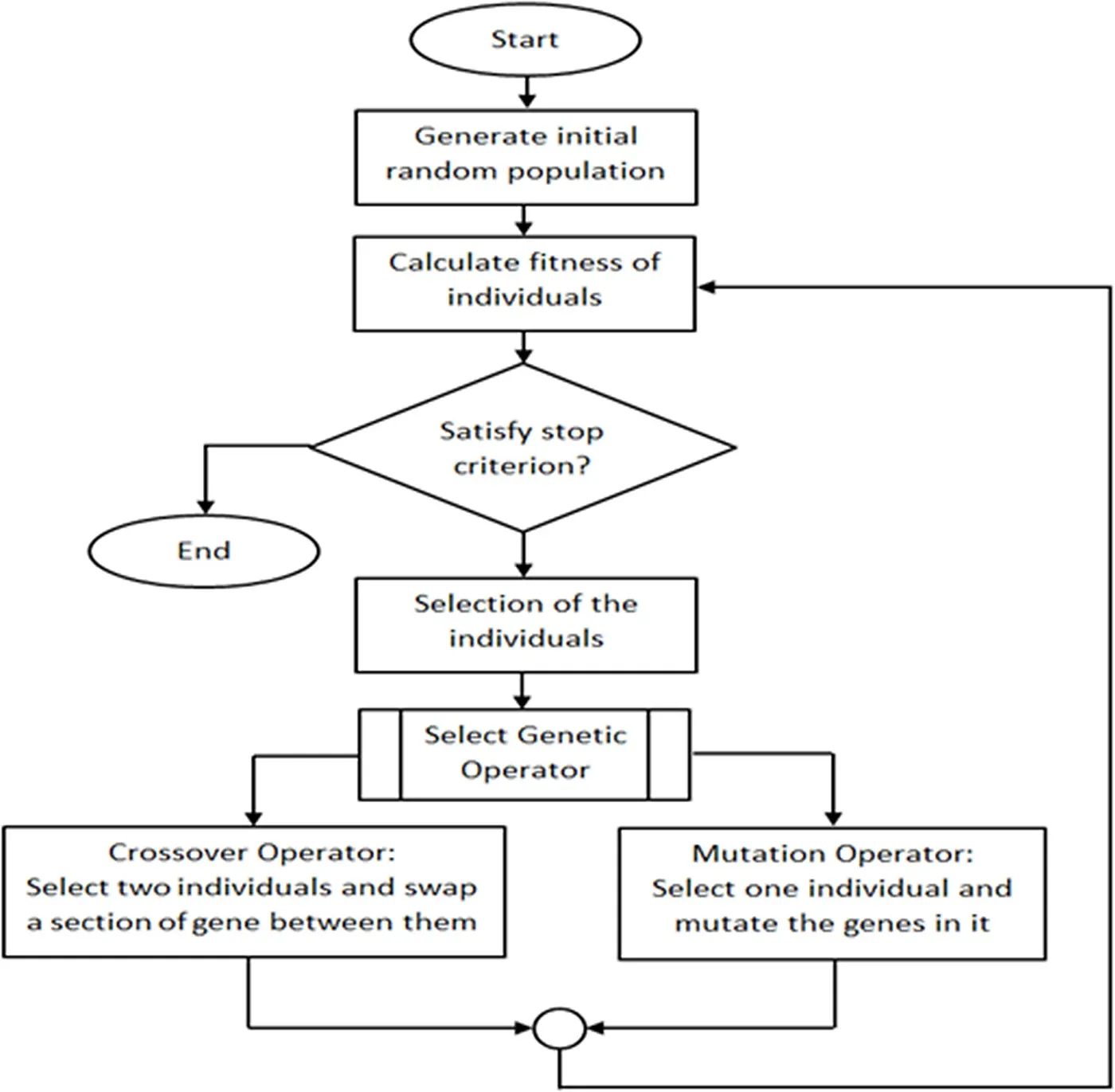
Steps involved in Genetic Algorithm,

• Starts with intialization of population.
• Next evaluate the fitness of each invidual.
• And select parents who is going to reproduce.
• Then crossover the mutation to the new one.
• And determine whic newbie is fittest.
• Then replace the existing solution newbies with fittest of previous got newbie.
• And repetation of above process till got finest newbie.

Syntax of Genetic Algorithm,

• x = ga(fun,nvars)
• x = ga(fun,nvars,A,b)
• x = ga(fun,nvars,A,b,Aeq,beq)
• x = ga(fun,nvars,A,b,Aeq,beq,lb,ub)
• x = ga(fun,nvars,A,b,Aeq,beq,lb,ub,nonlcon)
• x = ga(fun,nvars,A,b,Aeq,beq,lb,ub,nonlcon,options)
• x = ga(fun,nvars,A,b,Aeq,beq,lb,ub,nonlcon,intcon)
• x = ga(fun,nvars,A,b,Aeq,beq,lb,ub,nonlcon,intcon,options)
• x = ga(problem)
• [x,fval] = ga(___)
• [x,fval,exitflag,output] = ga(___)
• [x,fval,exitflag,output,population,scores] = ga(___)

Referwnce- https://in.mathworks.com/help/gads/ga.html

Main code,

Function code,

• Here we use this formula to get a stalagmite function to plot the main function.

function [globe] = stalagmite_func(vector)

x = vector(1);

y = vector(2);

f1x=(sin(5.1*pi*vector(1)+0.5)).^6;

f1y=(sin(5.1*pi*vector(2)+0.5)).^6;

f2x=exp((-4*log(2))*(vector(1)-0.0667).^2/0.64);

f2y=exp((-4*log(2))*(vector(2)-0.0667).^2/0.64);

globe = -(f1x*f1y*f2x*f2y);

end

Code explanation,

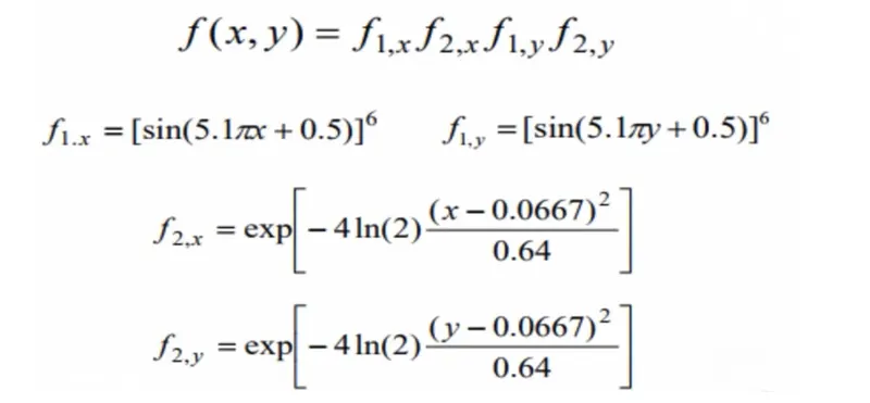
• Starts with clear all and close all and clc.
• First need to give inputs.That's variables name called x & y then give the linspace command value of 0-0.6 of 150 times.
• Then add the num of cases to 50 times and and craete 2d mesh using meshgrid command for the x & y input to the xx & yy output.
• Then starting iteration for evaluating the function cod and here i=length of xx and j=1:lenghth of yy then add the inputs of 1 & 2 = xx(i,j) & yy(i,j) like wise.
• And finally consider a function of i,j is equals to stalagmite_function (function code of stalagmite). of inputs.

Now see the studies about stalagmite.

Study 1- Statistical behaviour,

• Here 1st use for loop command for behaviour of bounds.
• And Store the X & Y values and then store the f optimum here.
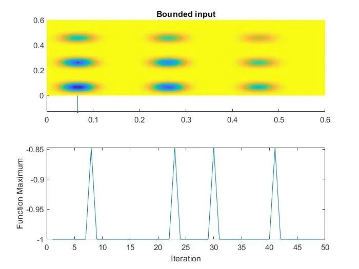
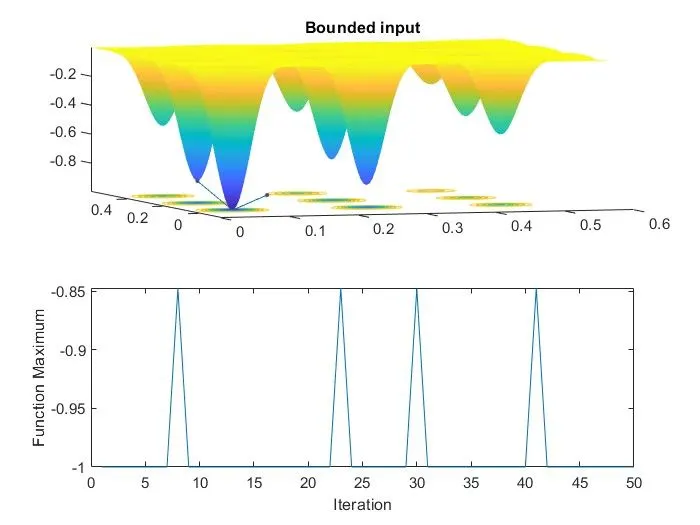
• Then use the ga command for this stalagmite function. the syntax was this one here x = ga(fun,nvars) finds a local unconstrained minimum, x, to the objective function, fun. nvars is the dimension (number of design variables) of function.
• And end this loop then add f=-f for plot comes stright for our reference.
• Here add the study1 time is toc and then give subplot to (2,1,1) for bounds in comes 3axis.
• Give shading interd command to see the plot clearly understand the bounds maximum minimum.
• Now plot3 to x output, y output, & f optimum this one comes 3axis view and also able to see 3d view of bounds.
• Then give the title and xlabel and ylabel names.
• Here code and result mentioned below.

%Study 1- Statistical behaviour

tic

for i=1:num_cases

[inputs,fopt(i)] = ga(@stalagmite_func,2);

xopt(i)=inputs(1);

yopt(i)=inputs(2);

end

fopt =-fopt;

f=-f;

study1_time = toc;

figure(1)

subplot(2,1,1);

hold on

surfc(xx,yy,f);

shading interp;

plot3(xopt,yopt,fopt,'Marker','o','MarkerSize',2,'MarkerfaceColor','r');

title('Unbounded input');

subplot(2,1,2);

plot(fopt);

xlabel('Iteration');

ylabel('Function minimum');

Results,

Study2-Stastical behaviour with upper limits and lower bounds,

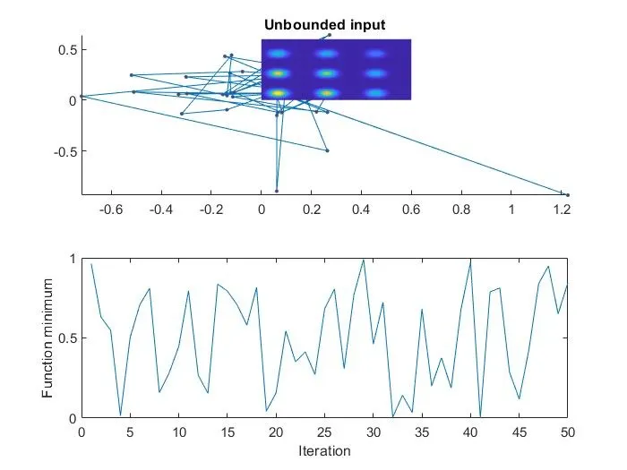
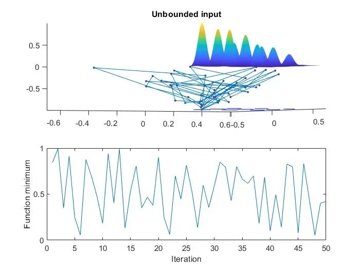
• Same as previous study for this one but here the syntax of ga was only going to change for upper and lower limits. x = ga(fun,nvars,A,b,Aeq,beq,lb,ub) defines a set of lower and upper bounds on the design variables, x, so that a solution is found in the range lb ≤ x ≤ ub.(Set A=[] and B=[] if no linear equalities exist.) (Set Aeq=[] and beq=[] if no linear equalities exist.).

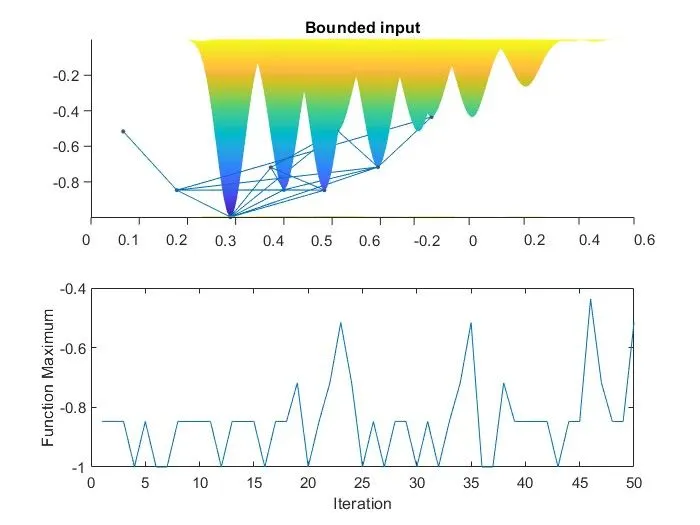
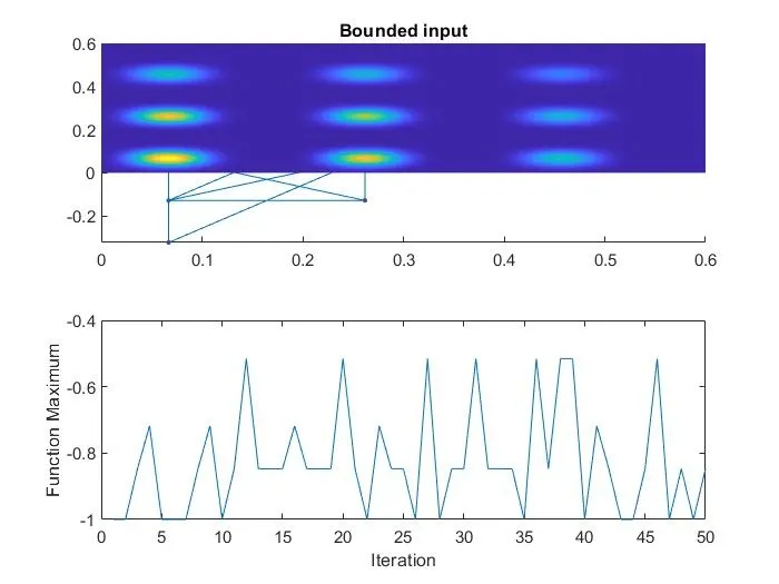
• Here also syntax of ga was only going to change and results will be get better.

Code,

Results,

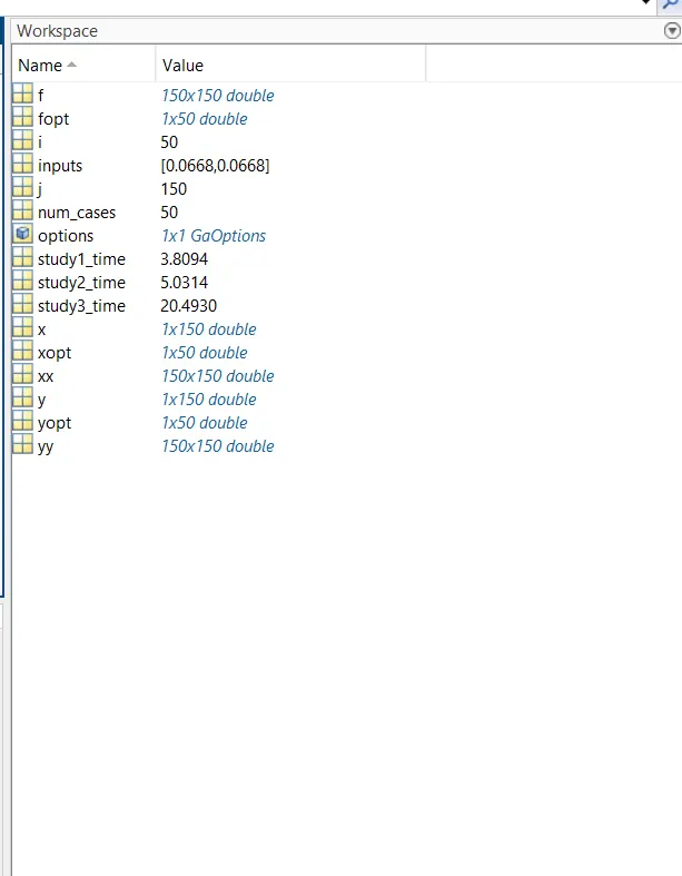
Work space results,

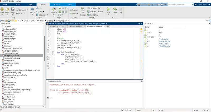
Errors facing while coding,

1st error- here I type the wrong spelling of inputs.

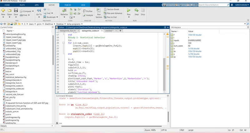
2nd error- In this wrongly spell the name of function

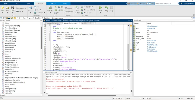
3rd error- Here type Marker face colour to instead of mareker colour

4th error- In this I forgot to add 4 brackets for non linear equalities.

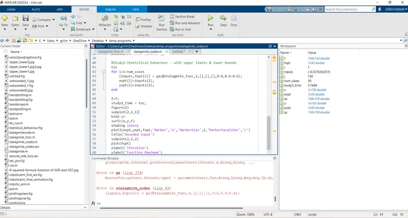
5th error-Here the optimoption spelling was correct.

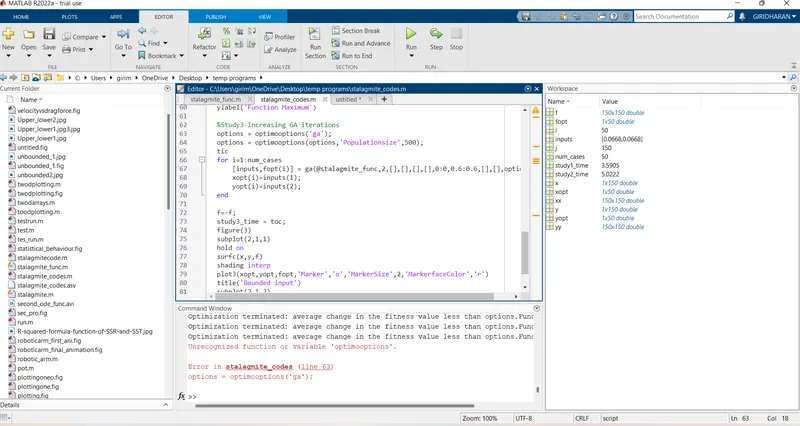
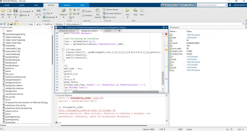
6th error-In this one I type 2 open brackets.

Conclusion,

• In this matlab coding easily understand about genetic algorithm and it's steps involved in programinng and how this is performs better options.