Week 3 - Solving second order ODEs
Aim,
- To create program for Ordinary Differential Equation for a simple pendulum.
- And create animation for simple pendulum motion.
Procedure,
The Ordinary Differential Equation is mentioned below,
In the above equation,
g = gravity in m/s2,
L = length of the pendulum in m,
m = mass of the ball in kg,
b=damping coefficient.
We could use this equation to create a program for pendulum,
in this we assume the values
L=1 metre,
m=1 kg,
b=0.05.
g=9.81 m/s2.
Step1,
- Here we see the 1st program.
- Here first we need to write the inputs.
- Then theta was angular displacement (is 0)and angular velocity (is 3) so we take the values of row matrix so we type in bracket with semi coloumn.
- Pendulum motion time is 0-20 sec so this is span time.And here hundreds values of ODE's need to be calculated so we use the linspace command for time array. t_span = linspace(0,20,500).
- And the ODE solving through the time with results that equation is [t,results] = ode45(@(t,theta) ode_func(t,theta,b,l,g,m),t_span by the coloumn of 500 values, theta_0 here, ode 45 is inbuilt command in matlab for ODE, and ode_func whose inputs are(t,theta,b,g,l,m) and span time and starting (angular displacement,angular velocity)called theta_0.
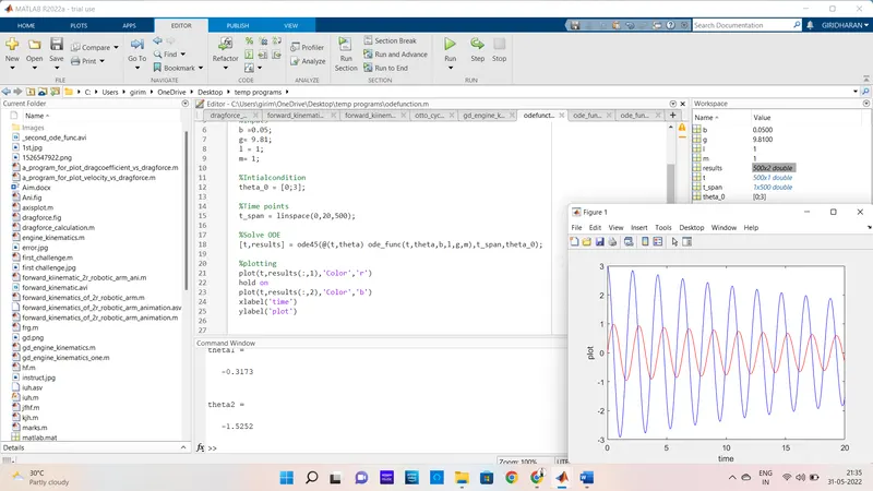
- Finally plotting was time and results.
Program1,
%inputs
b =0.05;
g= 9.81;
l = 1;
m= 1;
%Intialcondition
theta_0 = [0;3];
%Time points
t_span = linspace(0,20,500);
%Solve ODE
[t,results] = ode45(@(t,theta) ode_func(t,theta,b,g,l,m),t_span,theta_0);
ct=1
plot(t,results(:,1),'Color','r')
hold on
plot(t,results(:,2),'Color','b')
xlabel('time')
ylabel('plot')
Step2,
- Now see the second program is a function program.
- 1st need to give name was a function.
- Here store the function[dtheta_dt] variables are t,theta,b,l,g,m.
- Storing the values of angular displacement as theta1 and angula velocity as theta2.
- Here dtheta1 is angular velocity so that is theta2.
- And split the ode equation to here and need to find the dtheta2/dt and the equation is dtheta2_dt= -(b/m)* theta2-(g/l)*sin(theta1).
- And finally we need the dtheta_dt so we just add dtheta1 and dtheta2 by coloumn matrix so that equation is dtheta_dt = [dtheta1_dt; dtheta2_dt].
- Then add this function into 1st program we get the results.
Program2,
function [dtheta_dt] = ode_func(t,theta,b,l,g,m)
theta1 = theta(1)
theta2 = theta(2)
dtheta1_dt =theta2;
dtheta2_dt= -(b/m)* theta2-(g/l)*sin(theta1);
dtheta_dt = [dtheta1_dt; dtheta2_dt];
end
Output,
Step-2,
Animate the simple pendulum
Procedure,
- Here program was same as to plotting.
- Then we split the figure 1 & 2
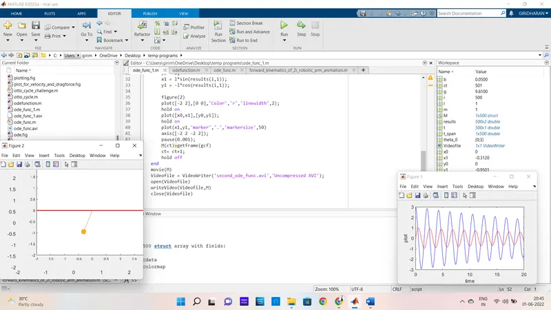
- Figure 2 is going to animation of pendulum.
- 1st we give the counter value as 1 then use the for loop command here.To make a motion of pendulum.
- And give length of rod.
- Then we give the coordinates x0,y0 values are 0.
- And x1 = l*cos(results(i,1)) & y1 = -l*cos(results(i,1)) for each repetition of for loop.
- Now plotting the co ordinattes of [-2 2],[0 0] with color of red and width of 2. and add hold on command to not erase the previous plot.
- Then plot for coordinates of x0,y0 & x1,y1 & and here also use Hold on command to not erase the previous plots.
- And give the axis-2to2 for X axis & Y axis.
- Then pause the loop to 0.001.
- And creating an array Mand store all the frames of the plot.
- Now increase counter value plus 1 for each reptition.
- End for loop
- And finally need to save the animation as video file.
- so create a movie and then it's a video file so write the video writter command and give name of a file(second_ode_func.avi) and it's need to be uncompressed.
- Then opening video file and create a video of each frames in the array M
- Last close the video file.
Program,
close all
clear all
clc
%inputs
b =0.05;
g= 9.81;
l = 1;
m= 1;
%Intialcondition
theta_0 = [0;3];
%Time points
t_span = linspace(0,20,500);
%Solve ODE
[t,results] = ode45(@(t,theta) ode_func(t,theta,b,l,g,m),t_span,theta_0);
figure(1)
plot(t,results(:,1),'Color','r')
hold on
plot(t,results(:,2),'Color','b')
xlabel('time')
ylabel('plot')
ct=1;
for i=1:length(t)
%pendulum motion
x0 = 0;
y0 = 0;
x1 = l*sin(results(i,1));
y1 = -l*cos(results(i,1));
figure(2)
plot([-2 2],[0 0],'Color','r','linewidth',2);
hold on
plot([x0,x1],[y0,y1]);
hold on
plot(x1,y1,'marker','.','markersize',50)
axis([-2 2 -2 2]);
pause(0.001);
M(ct)=getframe(gcf)
ct= ct+1;
hold off
end
movie(M)
Videofile = VideoWriter('second_ode_func.avi','Uncompressed AVI');
open(Videofile)
writeVideo(Videofile,M)
close(Videofile)
Output,
Here is the animation of the simple pendulum.
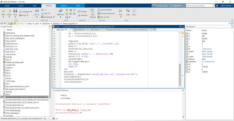
and programming screen shot.
Errors I faced,
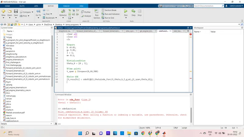
1st error- I didn't complete the program before itself I run it.
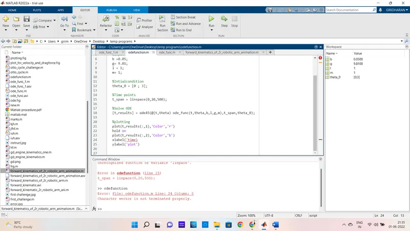
2nd error- In the xlabel i didn't add upper gamma.
3rd Error- In this I made function program mistake so this one comes an error.
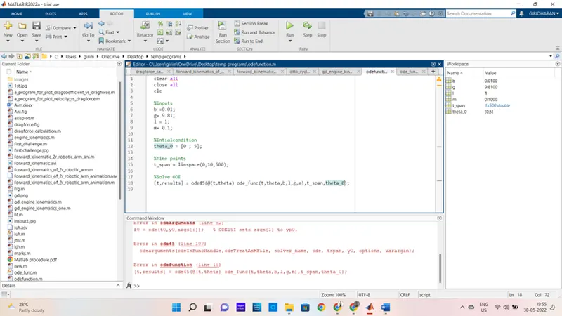
4th error - In this function program this no need to run that because all inputs are we give in main program.
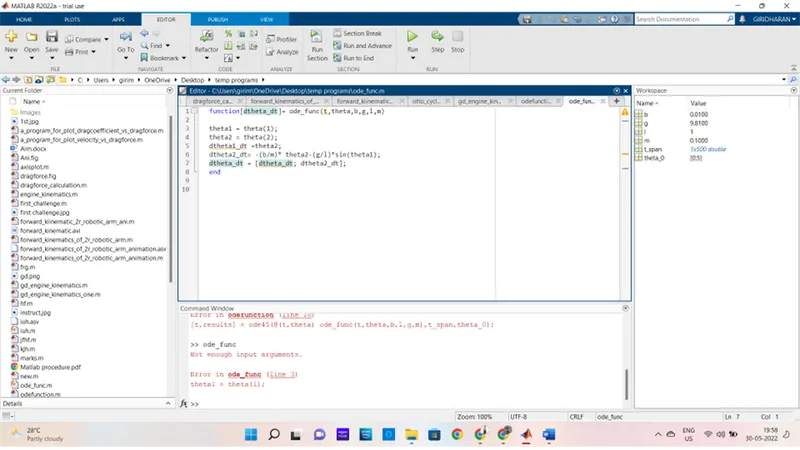
5th error - Here linewidth no need space.
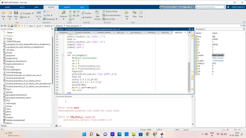
6th error - In this one pendulum upside is facing so we need to change x1 = -l*cos(results(i,1) them pendulum motion comes downside facing & another one is getframe means need to give video file then only this error not comes.
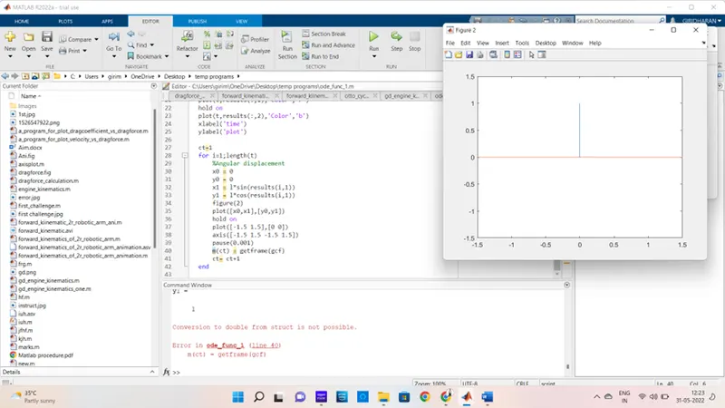
7th error - Here I was written the line 50 was write vido so correct this.
Conclusion,
1st was sucessfukky created a program for ordinary differential equation program.and animation was created for simple pendulum also created sucessfully using MATLAB.