Challenge

Project 2 - Rankine cycle Simulator

GGiridharan Ms21 Jul 2022

MATLAB

Aim,

Create a Rankine Cycle Simulator using MATLAB.
Calculate the state points of the Rankine Cycle based on inputs.
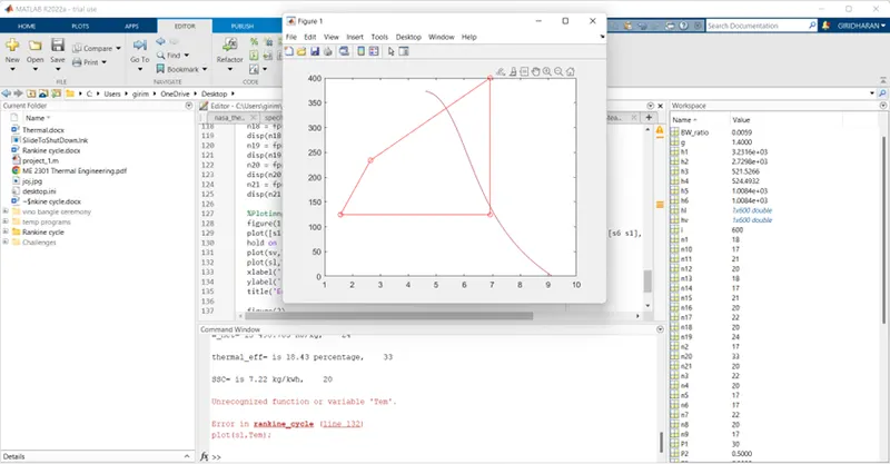
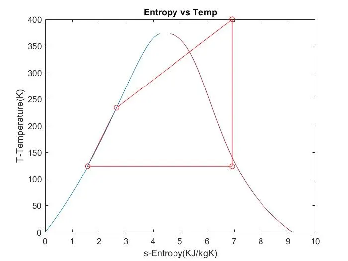
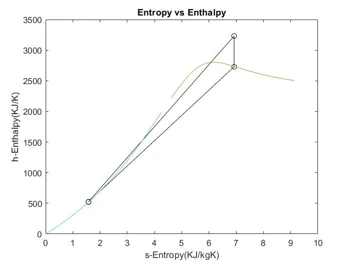
Plot the corresponding T-s and h-s plots for the given set of inputs. Title and axes labels are a must, while legends could be used if necessary.

Rankine cycle,

The Rankine cycle, also called the Rankine vapor cycle, is a thermodynamic cycle that converts a heat into mechanical energy.
A Rankine cycle is an ideal cycle which governs the working of a heat engine. There are four different components which works on different processes. They are turbine, condensor, pump and boiler.

Heat engine works with Rankine Cycle Model,

Rankine cycle process,

Process 1–2 is Isentropic Expansion in the turbine - Isentropic expansion of the working fluid through the turbine from saturated vapour at state 1 to the condenser pressure
Process 2–3 is Constant pressure heat rejection in the condensor- Heat transfer from the working fluid as it flows at constant pressure through the
condenser with saturated liquid at state 3.
Process 3–4 is Isentropic Expansion in the Pump- Isentropic compression in the pump to state 4 in the compressed liquid region.
Process 4–1 is Constant Presure & Heat addition to the Boiler- Heat transfer to the working fluid as it flows at constant pressure through the
boiler to complete the cycle.

Basic T-S & H-S Diagram,

Thermo dynamic Equations,

Process 1-2:Turbine Work-Isentropic expansion (𝐬𝟏 = 𝐬𝟐)

𝐖𝐓 = 𝐡𝟏 − 𝐡𝟐 (𝐤𝐉/𝐤𝐠)

h1 − Turbine inlet (𝐰𝐞𝐭 𝐨𝐫 𝐝𝐫𝐲 𝐨𝐫 𝐬𝐮𝐩𝐞𝐫𝐡𝐞𝐚𝐭𝐞𝐝 𝐬𝐭𝐞𝐚𝐦) enthalpy.

h2 − Turbine exit and condenser intet (𝐰𝐞𝐭 𝐨𝐫 𝐝𝐫𝐲 𝐬𝐭𝐞𝐚𝐦) enthalpy.

Process 2-3: Condenser heat rejection : Constant pressure heat rejection ( wet or dry steam convert
into liquid)

( 𝐏𝟐 = 𝐏𝟑)

𝐐𝐑 = 𝐡𝟐 − 𝐡𝟑 (𝐤𝐉𝐤𝐠)

h3 = hf2 = hf3 Condenser exit and pump inlet (saturated liquid) enthalpy

Process 3-4: Pump Work: Reversible adiabatic pumping (𝐬𝟑 = 𝐬𝟒)

𝐖𝐩 = 𝐡𝟑 − 𝐡𝟒 (𝐤𝐉𝐤𝐠)

h4 − Pump exit & boiler inlet (subcooled liquid) enthalpy

𝐖𝐩 = 𝑽𝒇𝟑(𝐏𝟒 − 𝐏𝟑 ) (𝐤𝐉𝐤𝐠)

𝐡𝟒 = 𝐖𝐩 + 𝐡𝟑 (𝐤𝐉𝐤𝐠)

Process 4-1: Boiler heat supplied (Constant pressure heat supplied) : Subcooled liquid to dry or
superheated steam ( 𝐏𝟒 = 𝐏𝟏)

𝐐𝐬 = 𝐡𝟏 − 𝐡𝟒 (𝐤𝐉𝐤𝐠)

Efficiency :

𝜼 =𝐖𝐓 − 𝐖𝐩

𝐐𝐬=(𝐡𝟏 − 𝐡𝟐) − (𝐡𝟑 − 𝐡𝟒 )

𝐡𝟏 − 𝐡2

For isentropic expansion:

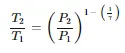
T = temperature at the state (K),

P = pressure at the state (Bar),

gamma = heat capacity ratio

For net work (W_net) and back work ratio (Bw_ratio):

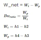
h = enthalpy at that state (kJ/kg)

W_t = turbine work (kJ/kg)

W_p = pump work (kJ/kg)

Thermal efficiency:

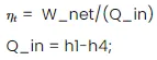
Q_in = heat added by the boiler (J)

Program,

clear all
close all
clc

%Inputs
disp('INPUTS')
P1 = 30;
T1 = 400;
P2 = 0.5;

disp('RANKINE CYCLE')
disp('1-2 is Isentropic Expansion in the turbine')
disp('2-3 is Constant pressure heat rejection in the condensor')
disp('3-4 is Isentropic Expansion in the Pump')
disp('4-1 is Constant Presure & Heat addition to the Boiler')


%Using Xsteam functions to find enthalpy and entropy at various points can be calculated
%Calculating enthalpy(h) and entropy(s) at state point 1
h1 = XSteam('h_pT',P1,T1);
s1 = XSteam('s_pT',P1,T1);

%Calculating Pressure(P),Enthalpy(h),and entropy(s) at state point 2
s2=s1;

%For Isentropic Expansion,(T2/T1)=(P2/P1)^(1-(1/g))
g=1.4;
power = 1-(1/g);
T2 = T1*((P2/P1)^power);
h2 = XSteam('h_PT',P2,T2);

%Calculating Pressure(P),Enthalpy(h),and entropy(s) at state point 3 
%since this process is constant pressure and heat removal
P3 = P2;
T3 = T2;
h3 = XSteam('hL_T',T3);
s3 = XSteam('sL_T',T3);

%Calculating Pressure(P),Enthalpy(h),and entropy(s) at state point 4 
%since Isentropic compression & Constan pressure
s4 = s3;
P4 = P1;
T4 = XSteam('T_ps',P4,s4);
h4 = XSteam('h_pT',P4,T4);
h5 = XSteam('hL_p',P4);
s5 = XSteam('sL_p',P4);
T5 = XSteam('T_hs',h5,s5);
h6 = XSteam('hL_p',P4);
s6 = XSteam('sL_p',P4);
T6 = XSteam('T_hs',h6,s6);

%Calciulating enr=tropy and enthalpy at the saturation curve
Temp = linspace(0,500,600);
for i = 1:length(Temp)
    sv(i) = XSteam('sv_T',Temp(i));
    sl(i) = XSteam('sl_T',Temp(i));
    hv(i) = XSteam('hv_T',Temp(i));
    hl(i) = XSteam('hl_T',Temp(i));
end

%Calculating net work out output (W_net) & back work ratio
W_t = h1-h2;
W_p = h4-h3;
W_net = W_t-W_p;
BW_ratio =W_p/W_t;

%Calculating thermal efficiency
Q_in = h1-h4;
thermal_eff = ((W_net/Q_in).*100);

%Calculating Specific steam consumption, 1J = 3600kg/s
SSC = 3600/W_net;

%Displaying results in command window
disp('Results')
disp('At stage point 1');
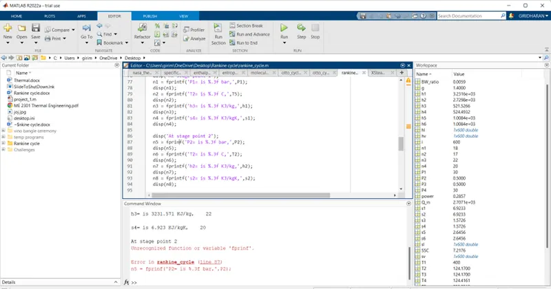
n1 = fprintf('P1= is %.3f bar,',P1);
disp(n1);
n2 = fprintf('T2= is %.3f C,',T5);
disp(n2);
n3 = fprintf('h3= is %.3f KJ/kg,',h1);
disp(n3);
n4 = fprintf('s4= is %.3f KJ/kgK,',s1);
disp(n4);

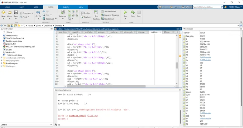
disp('At stage point 2');
n5 = fprintf('P2= is %.3f bar,',P2);
disp(n5);
n6 = fprintf('T2= is %.3f C,',T2);
disp(n6);
n7 = fprintf('h2= is %.3f KJ/kg,',h2);
disp(n7);
n8 = fprintf('s2= is %.3f KJ/kgK,',s2);
disp(n8);

disp('At stage point 3');
n9 = fprintf('P3= is %.3f bar,',P3);
disp(n9);
n10 = fprintf('T3= is %.3f C,',T3);
disp(n10);
n11 = fprintf('h3= is %.3f KJ/kg,',h3);
disp(n11);
n12 = fprintf('s3= is %.3f KJ/kgK,',s3);
disp(n12);

disp('At stage point 4');
n13 = fprintf('P4= is %.3f bar,',P4);
disp(n13);
n14 = fprintf('T4= is %.3f C,',T4);
disp(n14);
n15 = fprintf('h4= is %.3f KJ/kg,',h4);
disp(n15);
n16 = fprintf('s4= is %.3f KJ/kgK,',s4);
disp(n16);

n17 = fprintf('W_t= is %.3f KJ/kg,',W_t);
disp(n17);
n18 = fprintf('W_p= is %.3f KJ/kg,',W_p);
disp(n18);
n19 = fprintf('W_net= is %.3f KJ/kg,',W_net);
disp(n19);
n20 = fprintf('thermal_eff= is %.2f percentage,',thermal_eff);
disp(n20);
n21 = fprintf('SSC= is %.2f kg/kwh,',SSC);
disp(n21);

%Plotinng
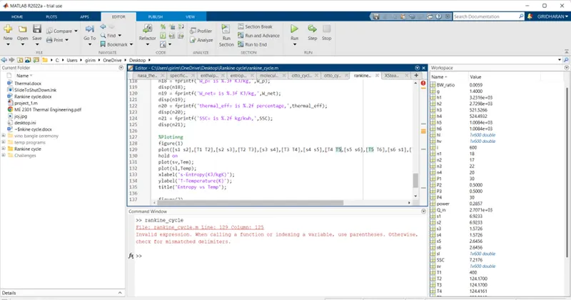
figure(1)
plot([s1 s2],[T1 T2],[s2 s3],[T2 T3],[s3 s4],[T3 T4],[s4 s5],[T4 T5],[s5 s6],[T5 T6],[s6 s1],[T6 T1],'marker','o','color','r')
hold on
plot(sv,Temp);
plot(sl,Temp);
xlabel('s-Entropy(KJ/kgK)');
ylabel('T-Temperature(K)');
title('Entropy vs Temp');

figure(2)
plot([s1 s2],[h1 h2],[s2 s3],[h2 h3],[s3 s4],[h3 h4],[s4 s1],[h4 h1],'marker','o','color','black');
hold on
plot(sv,hv);
plot(sl,hl);
xlabel('s-Entropy(KJ/kgK)');
ylabel('h-Enthalpy(KJ/K)');
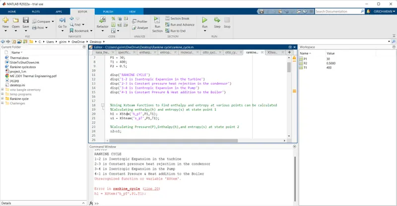
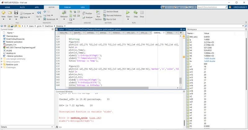
title('Entropy vs Enthalpy')

Program Explanation,

First start with the clear all,close all and clc.Then give the Inputs of Temperature and pressure,Then enter the display command to the process of Rankinne cycle.That code was

disp('RANKINE CYCLE')

disp('1-2 is Isentropic Expansion in the turbine')

disp('2-3 is Constant pressure heat rejection in the condensor')

disp('3-4 is Isentropic Expansion in the Pump')

disp('4-1 is Constant Presure & Heat addition to the Boiler')
After using XSteam function(Xsteam library) to find enthalpy and entropy at various points can be calculated.
Now we take enthalpy(h) and entropy(s) to be calculate at state point 1. That codes are,

h1 = XSteam('h_pT',P1,T1);

s1 = XSteam('s_pT',P1,T1);
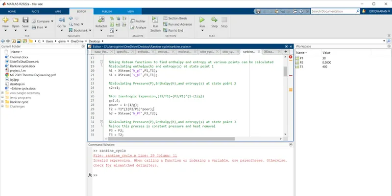
Similarly as Calculate the entropy and enthalpy and pressure at state point 2,Code was

%Calculating Pressure(P),Enthalpy(h),and entropy(s) at state point 2

s2=s1;

%For Isentropic Expansion,(T2/T1)=(P2/P1)^(1-(1/g))

g=1.4;

power = 1-(1/g);

T2 = T1*((P2/P1)^power);

h2 = XSteam('h_PT',P2,T2);

Here T2 need calculated means we use the this formula.
And Calculate the entropy and enthalpy and pressure at state point 3 & 4 that code was

%Calculating Pressure(P),Enthalpy(h),and entropy(s) at state point 3

%since this process is constant pressure and heat removal

P3 = P2;

T3 = T2;

h3 = XSteam('hL_T',T3);

s3 = XSteam('sL_T',T3);

%Calculating Pressure(P),Enthalpy(h),and entropy(s) at state point 4

%since Isentropic compression & Constan pressure

s4 = s3;

P4 = P1;

T4 = XSteam('T_ps',P4,s4);

h4 = XSteam('h_pT',P4,T4);

h5 = XSteam('hL_p',P4);

s5 = XSteam('sL_p',P4);

T5 = XSteam('T_hs',h5,s5);

h6 = XSteam('hL_p',P4);

s6 = XSteam('sL_p',P4);

T6 = XSteam('T_hs',h6,s6);
Then we need to calculate enthalpy and entropy was saturation curve,That code was,

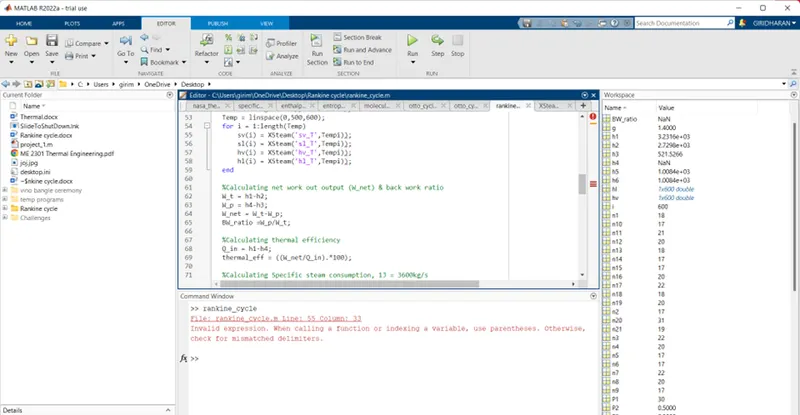
%Calculating enrtropy and enthalpy at the saturation curve

Temp = linspace(0,500,600);

for i = 1:length(Temp)

sv(i) = XSteam('sv_T',Temp(i));

sl(i) = XSteam('sl_T',Temp(i));

hv(i) = XSteam('hv_T',Temp(i));

hl(i) = XSteam('hl_T',Temp(i));

end
And calculate the work output,Thermal efficiency and Spcific steam consumption that code was mention below,

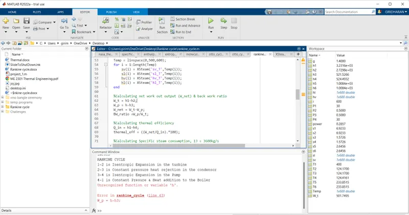
%Calculating net work out output (W_net) & back work ratio

W_t = h1-h2;

W_p = h4-h3;

W_net = W_t-W_p;

BW_ratio =W_p/W_t;

%Calculating thermal efficiency

Q_in = h1-h4;

thermal_eff = ((W_net/Q_in).*100);

%Calculating Specific steam consumption, 1J = 3600kg/s

SSC = 3600/W_net;
After that displayed the results in command window so we use these codes to get the results

%Displaying results in command window

disp('Results')

disp('At stage point 1');

n1 = fprintf('P1= is %.3f bar,',P1);

disp(n1);

n2 = fprintf('T2= is %.3f C,',T5);

disp(n2);

n3 = fprintf('h3= is %.3f KJ/kg,',h1);

disp(n3);

n4 = fprintf('s4= is %.3f KJ/kgK,',s1);

disp(n4);

disp('At stage point 2');

n5 = fprintf('P2= is %.3f bar,',P2);

disp(n5);

n6 = fprintf('T2= is %.3f C,',T2);

disp(n6);

n7 = fprintf('h2= is %.3f KJ/kg,',h2);

disp(n7);

n8 = fprintf('s2= is %.3f KJ/kgK,',s2);

disp(n8);

disp('At stage point 3');

n9 = fprintf('P3= is %.3f bar,',P3);

disp(n9);

n10 = fprintf('T3= is %.3f C,',T3);

disp(n10);

n11 = fprintf('h3= is %.3f KJ/kg,',h3);

disp(n11);

n12 = fprintf('s3= is %.3f KJ/kgK,',s3);

disp(n12);

disp('At stage point 4');

n13 = fprintf('P4= is %.3f bar,',P4);

disp(n13);

n14 = fprintf('T4= is %.3f C,',T4);

disp(n14);

n15 = fprintf('h4= is %.3f KJ/kg,',h4);

disp(n15);

n16 = fprintf('s4= is %.3f KJ/kgK,',s4);

disp(n16);

n17 = fprintf('W_t= is %.3f KJ/kg,',W_t);

disp(n17);

n18 = fprintf('W_p= is %.3f KJ/kg,',W_p);

disp(n18);

n19 = fprintf('W_net= is %.3f KJ/kg,',W_net);

disp(n19);

n20 = fprintf('thermal_eff= is %.2f percentage,',thermal_eff);

disp(n20);

n21 = fprintf('SSC= is %.2f kg/kwh,',SSC);

disp(n21);

Here we can use the n is variables to easily identify that names
Then plot the Temperature vs Entropy and Enthalpy vs Entropy the code was

%Plotinng

figure(1)

plot([s1 s2],[T1 T2],[s2 s3],[T2 T3],[s3 s4],[T3 T4],[s4 s5],[T4 T5],[s5 s6],[T5 T6],[s6 s1],[T6 T1],'marker','o','color','r')

hold on

plot(sv,Temp);

plot(sl,Temp);

xlabel('s-Entropy(KJ/kgK)');

ylabel('T-Temperature(K)');

title('Entropy vs Temp');

figure(2)

plot([s1 s2],[h1 h2],[s2 s3],[h2 h3],[s3 s4],[h3 h4],[s4 s1],[h4 h1],'marker','o','color','black');

hold on

plot(sv,hv);

plot(sl,hl);

xlabel('s-Entropy(KJ/kgK)');

ylabel('h-Enthalpy(KJ/K)');

title('Entropy vs Enthalpy')
Finished the code.

Output of T-S & H-S Diagram,

Command window Results,

INPUTS
RANKINE CYCLE
1-2 is Isentropic Expansion in the turbine
2-3 is Constant pressure heat rejection in the condensor
3-4 is Isentropic Expansion in the Pump
4-1 is Constant Presure & Heat addition to the Boiler
Results
At stage point 1
P1= is 30.000 bar,    18

T2= is 233.851 C,    17

h3= is 3231.571 KJ/kg,    22

s4= is 6.923 KJ/kgK,    20

At stage point 2
P2= is 0.500 bar,    17

T2= is 124.170 C,    17

h2= is 2729.822 KJ/kg,    22

s2= is 6.923 KJ/kgK,    20

At stage point 3
P3= is 0.500 bar,    17

T3= is 124.170 C,    17

h3= is 521.527 KJ/kg,    21

s3= is 1.573 KJ/kgK,    20

At stage point 4
P4= is 30.000 bar,    18

T4= is 124.416 C,    17

h4= is 524.493 KJ/kg,    21

s4= is 1.573 KJ/kgK,    20

W_t= is 501.750 KJ/kg,    22

W_p= is 2.967 KJ/kg,    20

W_net= is 498.783 KJ/kg,    24

thermal_eff= is 18.43 percentage,    33

SSC= is 7.22 kg/kwh,    20

>>

Errors I faced while coding,

1st - In this one line 20 Iwrongly type the XSteam