Week 4.1 - Genetic Algorithm
Writing a code to optimise the stalagmite function and find the global maxima of the function.
Using the genetic algorithm concept to find the optimum values using the stalagmite function
Explanation:
1. First, giving the input values x and y ranging from 0 to 1, having 100 values between 0 to 1
2. The number of iterations is given as 100
3. creating a 2d mesh for x and y values using meshgrid command
4. Now, define the function in the new tab. The function name is defined as the stalagmite function.
5. After defining the function command, we now use the' for' loop in the main code.
6. In the 'for' loop the x and y values in the 2d array are used to calculate the function f.
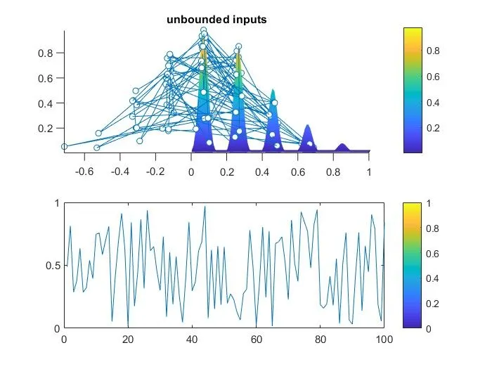
7. In the study1, using the for loop to find the statistical behaviour of the genetic algorithm.
8. In the previous for loop we have got the random values for x and y values. In order to get the optimum values, we are doing the study 1,2 and 3.
9. The genetic algorithm syntax is as follows in the code.
10. The genetic algorithm uses the stalagmite function and finds the minimum values of the two variables x and y for 100 iterations.
11. Now to find the maximum value of the negative of the function is used as the genetic algorithm only gives the minimum value.
12. Now we plot the optimum values of x,y and the function f.
13. In order to remove the lines in the graph we include the shading command
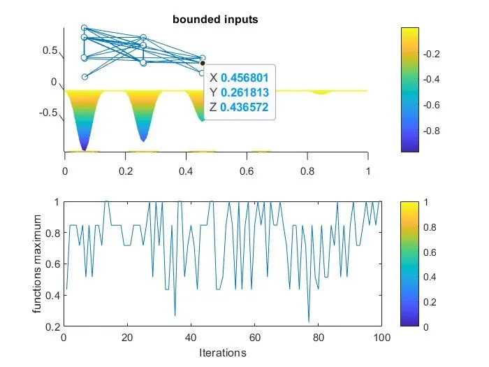
14. Now in the study2 we increase the population size from 100 to 200. For 200 iterations the genetic algorithm uses the stalagmite function and finds the optimum values for x,y and function f.
15. In study2 the syntax for genetic algorithm varies. The explanation for the syntax is as follows.
x = ga(fun,nvars,A,b,Aeq,beq,lb,ub,nonlcon)nonlcon. The function nonlcon accepts x and returns vectors C and Ceq, representing the nonlinear inequalities and equalities respectively. ga minimizes the fun such that C(x) ≤ 0 and Ceq(x) = 0. (Set lb=[] and ub=[] if no bounds exist.)
Note: This explanation is found in the Matlab documentation.
16. similarly in the study3 syntax for the genetic algorithm is as follows:
x = ga(fun,nvars,A,b,Aeq,beq,lb,ub,nonlcon,options)options. (Set nonlcon=[] if no nonlinear constraints exist.) Create options using optimoptions.
Note: This explanation is found in the Matlab documentation.
17. The optimum values of x,y and function f are plotted for study2 and study3.
18. compared to study1 and study2, the plot for the study3 is much neater
The code for the above explanation is given below.
clear all
close all
clc

%defining our search space
%vlaues for X and Y
%using linspace command
x = linspace(0,1,100)
y = linspace(0,1,100)

%number of iterations to be performed
num_cases = 100

%creating a 2d mesh
[xx yy] = meshgrid(x,y)

%using for loop
%for loop for x values
for i=1:length(xx)
    %for loop for y values
    for j = 1:length(yy)
        input(1)=xx(i,j)
        input(2)=yy(i,j)
        f(i,j)=stalagmite_fun(input)
    end
end

%study 1
%statistical behaviour of genetic algorithm
%using tic toc command to find the time taken to perform the iterations
tic
for i=1:num_cases
    %using genetic algorithm syntax
    [input,fopt(i)] = ga(@stalagmite_fun,2)

    %finding optimum values for x and y
    xopt(i)=input(1)
    yopt(i)=input(2)
end

%syntax for plotting maximum value of the function
fopt = -fopt
f = -f
study1_time = toc

%plotting study1
figure(1)
subplot(2,1,1)
hold on

%surface command for the plot
surfc(x,y,f)

%shading the graph using shading command
shading interp

%plot of x,y and function optimum values
plot3(xopt,yopt,fopt,'marker','o','MarkerSize',5,'MarkerFaceColor','auto')

%tittle of the plot
title('unbounded inputs')
subplot(2,1,2)
plot(fopt)
%labelling x and y axis
xlabel('Iterations')
ylabel('functions maximum')

%study2
%increasing the iteration values from 100 to 200
options = optimoptions('ga')
options = optimoptions(options,'PopulationSize',200)

tic
for i=1:num_cases
    %syntax for genetic algorithm
    [input,fopt(i)] = ga(@stalagmite_fun,2,[],[],[],[],[0:0],[1:1])
    %optimum values for x and y
    xopt(i)=input(1)
    yopt(i)=input(2)
end

%syntax for plotting maximum value of the function
fopt = -fopt
f = -f
study2_time = toc

%plotting study2
figure(2)
subplot(2,1,1)
hold on
%surface command for the plot
surfc(x,y,f)
%shading the graph using shading command
shading interp
%plot of x,y and function optimum values
plot3(xopt,yopt,fopt,'marker','o','MarkerSize',5,'MarkerFaceColor','auto')
%tittle of the plot
title('bounded inputs')
subplot(2,1,2)
plot(fopt)
%labelling x and y axis
xlabel('Iterations')
ylabel('functions maximum')

%study 3
%increasing the iteration values from 100 to 200
options = optimoptions('ga')
options = optimoptions(options,'PopulationSize',200)
tic
for i = 1:num_cases
    %syntax for genetic algorithm
    [input,fopt(i)] = ga(@stalagmite_fun,2,[],[],[],[],[0:0],[1:1],[],[],options)
    %optimum values for x and y
    xopt(i)=input(1)
    yopt(i)=input(2)
end

%syntax for plotting maximum value of the function
fopt = -fopt
f = -f
study3_time = toc

%plotting study3
figure(3)
subplot(2,1,1)
hold on
%surface command for the plot
surfc(x,y,f)
%shading the graph using shading command
shading interp
%plot of x,y and function optimum values
plot3(xopt,yopt,fopt,'marker','o','MarkerSize',5,'MarkerFaceColor','auto')
%tittle of the plot
title('bounded inputs')
subplot(2,1,2)
plot(fopt)
%labelling x and y axis
xlabel('Iterations')
ylabel('functions maximum')
using the function command
%using function command
%defining the function name
%finding the stalagmite function with x and y values
function f = stalagmite_fun(input)
         x = input(1)
         y = input(2)
        %solving the given formula
         f1x = (sin(((5.1*pi).*x)+0.5)).^6
         f1y = (sin(((5.1*pi).*y)+0.5)).^6

         f2x = exp((((x-0.0667).^2).*(-4*log(2)))./0.64)
         f2y = exp((((y-0.0667).^2).*(-4*log(2)))./0.64)
        %value of f
         f = -f1x*f1y*f2x*f2y
end
The plot for study1,study2 and study3 are as follows:
As the number of iterations increases the maximum value tends to be a single value.