Week 3 - Solving second order ODEs

The program for the equation of motion of a simple pendulum with damping is as follows:

clear all 
close all
clc

%solving a second order differential equation
%inputs
%damping coefficient,acceleration due to gravity,length of pendulum,mass of
%the ball
b = 0.05
g = 9.81
l = 1
m = 1

%initial conditioins
%initial displacement and initial velocity
theta_0 = [0;5]

%time points
t_span = linspace(0,20,750)

%solving ode
[t , results] = ode45(@(t,theta) ode_func(t,theta,b,g,l,m),t_span,theta_0)

%plotting
figure(1)
%plotting results with respect to displacement
plot(t,results(:,1))
hold on
%plotting results with respect to velocity
plot(t,results(:,2))
%labelling x-axis and y-axis
xlabel('time')
ylabel('plot')

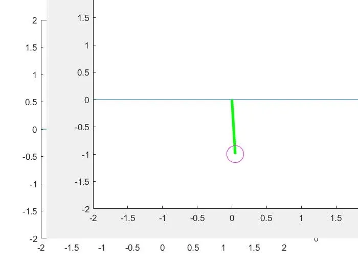
%Animation of pendulum
ct=1
figure(2)
%using for loop
for i=1:length(results(:,1))
%inputs
%defining origin and finding x1 and y1
    x_0 = 0
    y_0 = 0
    x_1 = l*sind(results(i,1))
    y_1 = -l*cosd(results(i,1))
%plotting
    plot([-2 2],[0 0])
    hold on
%plotting x0 y0 and x1 y1
    plot([x_0 x_1],[y_0 y_1],'linewidth',3,'color','g')
%axis for the plot
    axis([-2 2 -2 2])
%plotting pendulum using x1 y1
    plot(x_1,y_1,'o','MarkerSize',20,'Color','m')
%labelling the plot
    xlabel('Animation of pendulum')
%creating movie frame
%using getframe command
    M(ct) = getframe(gcf)
    hold off
    ct = ct+1
end

%making a movie file
movie(M)
%creating a videofile and saving the animation video
videofile = VideoWriter('simple_pendulum.avi')
open(videofile)
writeVideo(videofile,M)
close(videofile)

using function command:

%using function command
%creating file name as function name
function [dtheta_dt] = ode_func(t,theta,b,g,l,m)
         %dividing second order ode into two first order ode
         theta1 = theta(1)
         theta2 = theta(2)
         %finding theta2 using dtheta1/dt
         dtheta1_dt = theta2
         %equation for solving dtheta2/dt
         dtheta2_dt = -(b/m)*theta2 - (g/l)*sind(theta1)
         %final theta value
         dtheta_dt = [dtheta1_dt; dtheta2_dt]
end
%end of function command

Explanation of the code:

1. The initial parameters required for solving the differential equation are damping coefficient(b), gravity(g), length of the pendulum(L) and mass of the ball(m).

2. The initial theta conditions for displacement and velocity are 0 and 5.

3. The time period of the pendulums is taken from 0 to 20secs with 750 values between zero to 20.

4. Now, the second-order differential equation is divided into two first-order differential equations by inputting theta values as theta1 and theta2.

5. In the function command all the input parameters are written on the right-hand side and the results are taken on the left-hand side.

6. By dividing the second-order differential equation we get the equation as -(b/m)*theta2 - (g/l)*sind(theta1).

7. This equation gives the theta2 value and the final value of theta is derived from both the theta1 and theta2 values.

8. Now plotting the results. The plot is made between the displacement and velocity with respect to theta.

9. In the first figure the curves between time and theta are plotted.

10. The animation of the simple pendulum is created using a for loop. Firstly the origin (0,0) is taken and x0 and y0.

11. The axis is taken from -2 to 2 for both X and Y axis. To find x1 and y1 we used the length of the pendulum and the theta values.

12. The equation for x1 and y1 are as follows.

x_1 = l*sind(results(i,1))

image of plot:

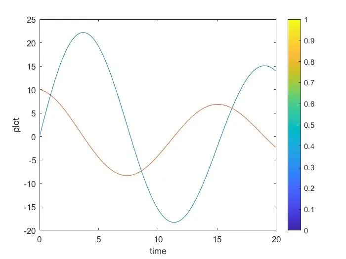
image of animation:

youtube link for animation:

https://youtu.be/TVoMo2txNgc