Week 3.5 - Deriving 4th order approximation of a 2nd order derivative using Taylor Table method

Aim:

To write a program to derive the fourth order approximation of a second derivative using central differencing scheme, skewed right sided differencing scheme and skewed left sided differencing scheme with the help of Taylor table method and to compare the analytical derivative with Truncation error.

Scheme Derivations:

Central Differencing Scheme:

No of Nodes:

The number of nodes = p +q-1

Where,

p is order of derivative.

q is order of approximation

The number of nodes = 2+4-1 = 5

Derivation:

Fourth order approximation for the second order derivative,

(∂^2 u)/(∂x^2 ) = (af(i-2)+bf(i-1)+cf(i)+df(i+1)+ef(i+2))/(dx^2) .......(1)

Taylor table method:

dx2f ՛՛(i)	f(i)	f ՛(i)dx	f ՛՛(i)dx2	f ՛՛՛(i)dx3	f ՛՛՛՛(i)dx4
af(i-2)	a	-2a	2a	-(4a/3)	2a/3
bf(i-1)	b	-b	b/2	-(-b/6)	b/24
cf(i)	c	0	0	0	0
df(i+1)	d	d	d/2	d/6	d/24
ef(i+2)	e	2e	2e	4e/3	2e/3
sum of co_efficients	0	0	1	0	0

A.X = B

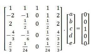
X = inv(A)*B

By solving the equation,

a = -0.0833, b = 1.3333, c = -2.5000, d = 1.3333, e = -0.0833

Substituting the above values in equation (1),

(∂^2 u)/(∂x^2 ) = ((-0.0833)f(i-2)+(1.3333)f(i-1)+(-2.5000)f(i)+(1.3333)f(i+1)+(-0.0833)f(i+2))/(dx^2) 

Skewed Right sided differencing Scheme:

No of Nodes:

The number of nodes = p +q

Where,

p is order of derivative.

q is order of approximation

The number of nodes = 2+4 = 6

Derivation:

Fourth order approximation for the second order derivative,

(∂^2 u)/(∂x^2 ) = (af(i)+bf(i+1)+cf(i+2)+df(i+3)+ef(i+4)+gf(i+5))/(dx^2)..... (2)

Taylor table method:

dx2f ՛՛(i)	f(i)	f ՛(i)dx	f ՛՛(i)dx2	f ՛՛՛(i)dx3	f ՛՛՛՛(i)dx4	f ՛՛՛՛՛(i)dx5
af(i)	a	0	0	0	0	0
bf(i+1)	b	b	b/2	b/6	b/24	b/120
cf(i+2)	c	2c	4c/2	8c/6	16c/24	32c/120
df(i+3)	d	3d	9d/2	27d/6	81d/24	243d/120
ef(i+4)	e	4e	16e/2	64e/6	256e/24	1024e/120
gf(i+5)	g	5g	25g/2	125g/6	625g/24	3125g/120
sum of co_efficients	0	0	1	0	0	0

A.X = B

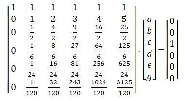
X = inv(A)*B

By solving the equation,

a = 3.7500, b = -12.8333, c = 17.8333, d = -13.0000, e = 5.0833, g = -0.8333

Substituting the above values in equation (2),

(∂^2 u)/(∂x^2 ) = ((3.7500)f(i)+(-12.833)f(i+1)+(17.8333)f(i+2)+(-13.000)f(i+3)+(5.0833)f(i+4)+(-0.8333)f(i+5))/(dx^2) 

Skewed Left sided differencing Scheme:

No of Nodes:

The number of nodes = p +q

Where,

p is order of derivative.

q is order of approximation

The number of nodes = 2+4 = 6

Derivation:

Fourth order approximation for the second order derivative,

(∂^2 u)/(∂x^2 ) = (af(i-5)+bf(i41)+cf(i-3)+df(i-4)+ef(i-5)+gf(i))/(dx^2)......(3)

Taylor table method:

dx2f ՛՛(i)	f(i)	f ՛(i)dx	f ՛՛(i)dx2	f ՛՛՛(i)dx3	f ՛՛՛՛(i)dx4	f ՛՛՛՛՛(i)dx5
af(i)	a	-5a	25a/2	-(125a/6)	625a/24	-(3125a/120)
bf(i+1)	b	-4b	16b/2	-( 64b/6)	256b/24	-(1024b/120)
cf(i+2)	c	-3c	9c/2	-( 27c/6)	81c/24	-(243c/120 )
df(i+3)	d	-2d	4d/2	-(8d/6)	16d/24	-(32d/120)
ef(i+4)	e	-e	e/2	-(e/6 )	e/24	-(e/120 )
gf(i+5)	g	0	0	0	0	0
sum of co_efficients	0	0	1	0	0	0

A.X = B

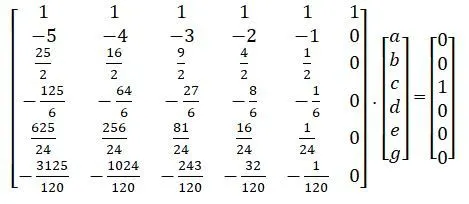
X = inv(A)*B

By solving the equation,

a = -0.8333, b = 5.0833, c = -13.0000, d = 17.8333, e = -12.8333, g = 3.7500

Substituting the above values in equation (2),

(∂^2 u)/(∂x^2 ) = ((-0.8333)f(i-5)+(5.0833)f(i-4)+(-13.0000)f(i-3)+(17.8333)f(i-2)+(-12.8333)f(i-1)+(3.7500)f(i))/(dx^2) 

Central Differencing Function Code:

function out_error_central = central_approximation(x,dx)
% f(x) = exp(x)*sin(x)
analytical_derivative = -2*exp(x)*sin(x)

central_differencing = (((-0.0833)*((exp(x-(2*dx)))*(cos(x-(2*dx)))))+((1.3333)*((exp(x-dx))*(cos(x-dx))))-((2.5000)*((exp(x))*(cos(x))))+((1.3333)*((exp(x+dx))*(cos(x+dx))))-((0.0833)*((exp(x+(2*dx)))*(cos(x+(2*dx))))))/(dx^2);

%error

out_error_central = abs(central_differencing-analytical_derivative)
end

Skewed Right sided differencing Function Code:

function out_error_right_sided_skew =right_sided_skew_approximation(x,dx);
% f(x) = exp(x)*sin(x)
analytical_derivative = -2*exp(x)*sin(x)

right_sided_skew_differencing = (((3.7500)*((exp(x))*(cos(x))))-((12.8333)*((exp(x+dx))*(cos(x+dx))))+((17.8333)*((exp(x+(2*dx)))*(cos(x+(2*dx)))))-((13.0000)*((exp(x+(3*dx)))*(cos(x+(3*dx)))))+((5.0833)*((exp(x+(4*dx)))*(cos(x+(4*dx)))))-((0.8333)*((exp(x+(5*dx)))*(cos(x+(5*dx))))))/(dx^2);

%error

out_error_right_sided_skew = abs(right_sided_skew_differencing-analytical_derivative)
end

Skewed Left sided differencing Function Code:

function out_error_left_sided_skew = left_sided_skew_approximation(x,dx)
% f(x) = exp(x)*sin(x)
analytical_derivative = -2*exp(x)*sin(x)

left_sided_skew_differencing = (((-0.8333)*((exp(x-(5*dx)))*(cos(x-(5*dx)))))+((5.0833)*((exp(x-(4*dx)))*(cos(x-(4*dx)))))-((13.0000)*((exp(x-(3*dx)))*(cos(x-(3*dx)))))+((17.8333)*((exp(x-(2*dx)))*(cos(x-(2*dx)))))-((12.8333)*((exp(x-dx))*(cos(x-dx))))+((3.7500)*((exp(x))*(cos(x)))))/(dx^2);

%error

out_error_left_sided_skew = abs(left_sided_skew_differencing-analytical_derivative)
end

Main Program:

clear all
close all
clc

x = pi/3;
dx = linspace(pi/40,pi/4000,20);

for i = 1:length(dx)
    central_differencing_error(i) = central_approximation(x,dx(i))
    right_sided_skew_differencing_error(i) = right_sided_skew_approximation(x,dx(i))
    left_sided_skew_differencing_error(i) = left_sided_skew_approximation(x,dx(i))
end


%plotting
loglog(dx,central_differencing_error,'r')
hold on
loglog(dx,right_sided_skew_differencing_error,'b')
hold on
loglog(dx,left_sided_skew_differencing_error,'g')
xlabel('dx')
ylabel('Error')
legend('Central Differencing','Skewed RIght Sided Differencing','Skewed Left Sided Differencing')

Code Explanation:

• Starting few commands like ‘clear all’, ‘close all’, ‘clc’ are entered to clear any existing data from previous program or command section.
• Then enter the input values like x and dx. Then create an individual function program to calculate centrl differencing, Skewed right sided differencing and Skewed right sided differencing.
• Then enter the formula to calculate error in each function, use the abs command that helps answer not to change when the order change during subtraction.
• Then call those function programs in main program to get the results.
• Then use the loglog command to plot and compare the results of error of each differencing approximation.
• Save and Run the program to get the results and plot.

Results:

Plot:

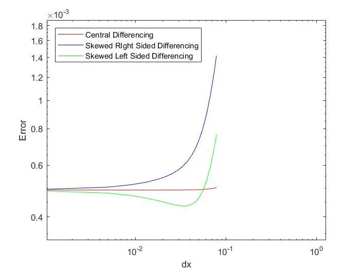
The above plot shows that the central differencing scheme has less error compare to other two shemes.