Week 4.1 - Genetic Algorithm
AIM:
- Write a code in MATLAB to optimise the stalagmite function and find the global maxima of the function.
OBJECTIVE:
- Clearly expalin the concept of genetic algorithm in your own words and also explain the syntax for 'ga' in MATLAB in your report.
- Make sure that your code gives the same output, even if it is made to run several times.
- Plot graphs for all 3 studies and for F maximum vs no. of iterations. Title and axes labels are a must, legends could be shown if necessary.
GENETIC ALGORITHM:
- The genetic algorithm is a technique for solving both constrained and unconstrained optimization problems that are based on natural selection, the process that drives biological evolution.
- Generates a population of points at each iteration. The best point in the population approaches an optimal solution.
STALAGMITE FUNCTION
- A stalagmite is a type of rock which is an upward-growing mound of mineral deposits that have precipitated from water dripping onto the floor of a cave.
- Like that we are going to create graph like the stalagmite based upon the Genetic algorithm.
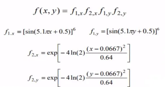
FORMULA:
FUNCTION PROGRAM:
function [f]=stalagmite(input_vector)

x=input_vector(1);
y=input_vector(2);

f1=(sin(5.1*pi*x+0.5))^6;
f2=(sin(5.1*pi*y+0.5))^6;
f3=exp(-4*log(2)*(x-0.0667)^2/0.64);
f4=exp(-4*log(2)*(y-0.0667)^2/0.64);

f=(-f1*f2*f3*f4);
end
EXPLANATION:
- This functiion program is used to set a template for the stalagmite formula to get assign in the genetic algorithm.
PROGRAM:
close all
clear all
clc

%Define the value of X and Y
x=linspace(0,0.6,150);
y=linspace(0,0.6,150);

%Creating an 2D Mesh
iterations= 150;
[xx,yy]= meshgrid(x,y);

%Evaluating the stalagmite function

for i=1:length(xx)
    for j=1:length(yy)
        input_vector(1)=xx(i,j);
        input_vector(2)=yy(i,j);
        f(i,j)=stalagmite(input_vector);
    end
end
tic
for i=1:iterations
    [input,f_opt(i)]=ga(@stalagmite,2);
    x_opt(i)=input(1);
    y_opt(i)=input(2);
end

iteration_1_time=toc

figure(1)
subplot(2,1,1)
hold on
surfc(xx,yy,-f)
shading interp
plot3(x_opt,y_opt,-f_opt,'marker','o','markersize',5,'markerfacecolor','g')
title('Unbounded inputs')
subplot(2,1,2)
plot(-f_opt)
xlabel('Iterations');
ylabel('Function Minimum');

tic
for i=1:iterations
    [input,f_opt(i)]=ga(@stalagmite,2,[],[],[],[],[0,0],[1,1]);
        x_opt(i)=input(1);
        y_opt(i)=input(2);
end

iteration_2_time=toc

figure(2)
subplot(2,1,1);
hold on
surfc(xx,yy,-f)
shading interp
plot3(x_opt,y_opt,-f_opt,'marker','o','markersize',5,'markerfacecolor','g')
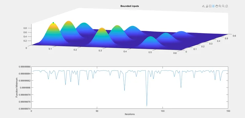
title('Bounded inputs')
subplot(2,1,2)
plot(-f_opt)
xlabel('Iterations')
ylabel('Function Minimum')

options=optimoptions('ga');
options=optimoptions(options,'populationsize',500);

tic
for i=1:iterations
    [input,f_opt(i)]=ga(@stalagmite,2,[],[],[],[],[0,0],[0.6,0.6],[],[],options);
        x_opt(i)=input(1);
        y_opt(i)=input(2);
end

figure(3)
subplot(2,1,1)
hold on
surfc(xx,yy,-f)
shading interp
plot3(x_opt,y_opt,-f_opt,'marker','o','markersize',5,'markerfacecolor','g')
title('Bounded inputs')
subplot(2,1,2)
plot(-f_opt)
xlabel('Iterations')
ylabel('Function Minimum')
SYNTAX OF GA USED IN THE PROGRAM:
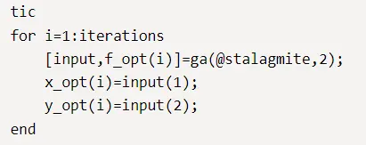
x= ga(fun,nvars)x, to the objective function,fun.nvarsis the dimension (number of design variables) offun.- As per the syntax of ga (@stalagmite,2) is which the stalagmite is an function and which 2 is used to show the variable used (x,y).
x =
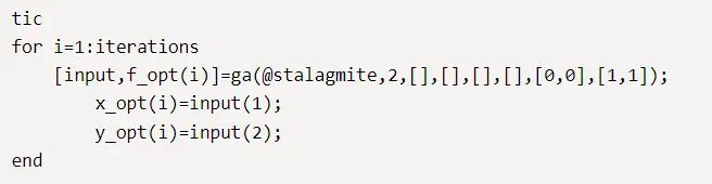
x = ga(defines a set of lower and upper bounds on the design variables,fun,nvars,A,b,Aeq,beq,lb,ub)x, so that a solution is found in the rangelb≤x≤ub. (SetAeq=[]andbeq=[]if no linear equalities exist.)- As per the syntax of ga which the function and variable fixed and the boundary setted for the program.
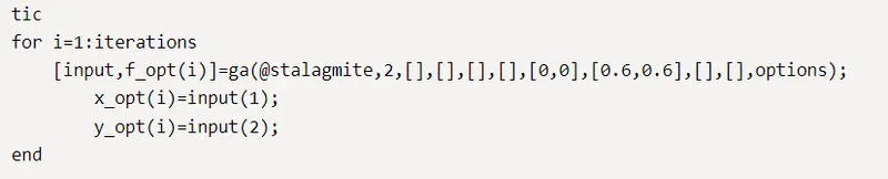
x= ga(fun,nvars,A,b,Aeq,beq,lb,ub,nonlcon,options)options. (Setnonlcon=[]if no nonlinear constraints exist.) Createoptionsusingoptimoptions.- As per the syntax of ga which a function,variable,boundary and options also used to create a gragh.
ERRORS:
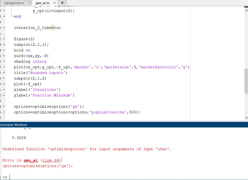
Error: Instead of optimoptions Ihave typed optimizeoptions
Action: The error has been corrected.
OUTPUT:
Figure 1
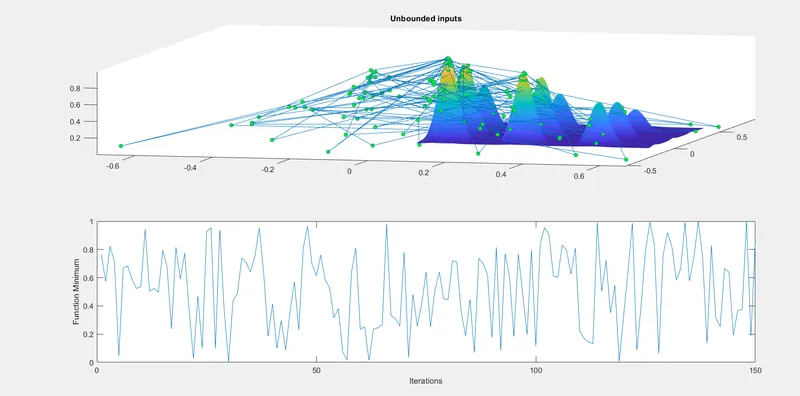
Figure 2
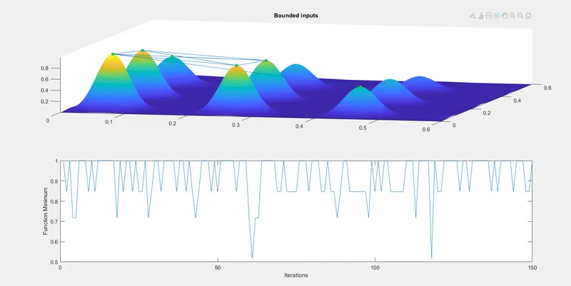
Figure 3