Week 3 - Solving second order ODEs

AIM:

Write a program in Matlab\Octave that will simulate the pendulum motion.

SECOND ORDER ODE:

• Second order differential equation is a specific type of differential equation that consists of a derivative of a function of order 2 and no other higher-order derivative of the function appears in the equation.

PENDULUM:

• A pendulum is a body suspended from a fixed point so that it can swing back and forth under the influence of gravity. The time interval of a pendulum’s complete back-and-forth movement is constant.
• The Simple Pendulum A simple pendulum consists of a mass m (of negligible size) suspended by a string or rod of length L (and negligible mass). The angle it makes with the vertical varies with time as a sine or cosine.

In the above equation,

• g = gravity in m/s2,
• L = length of the pendulum in m,
• m = mass of the ball in kg,
• b = damping coefficient.

GIVEN DATA:

1. L = 1 metre
2. m = 1 kg
3. b = 0.05
4. g = 9.81 m/s2
5. Angular displacement = 0
6. Angular velocity = 3 rad/sec

FUNCTIONAL PROGRAM:

function [dtheta_dt]=ode_func(t,theta,b,g,l,m)
theta1=theta(1);
theta2=theta(2);
dtheta1_dt=theta2;
dtheta2_dt=-(b/m)*theta2-(g/l)*sin(theta1);
[dtheta_dt]=[dtheta1_dt;dtheta2_dt];
end

FUNCTION EXPLANATION:

• This is the program to calculate the ODE equation of simple pendulum with damping.
• This is which we have created a template to calculate the equation of motion of a simple pendulum with damping.

SECOND ORDER ODE PROGRAM FOR PENDULUM MOVEMENT:

close all
clear all
clc
b=0.05;
g=9.81;
l=1;
m=1;

%initial_condition
theta_0=[0;3];

%time_points
t_span=linspace(0,5,25);

%solve_ode
[t,result]=ode45(@(t,theta) ode_func(t,theta,b,g,l,m),t_span,theta_0);
y = result(:,1);
plot(t,result(:,1))
hold on
plot(t,result(:,2))
xlabel('time');
ylabel('plot')
grid on
hold off

ct=1;
for i=1:length(t_span)
    
    x0=0;
    y0=0;
    
    x1= l*sin(y(i));
    y1=-l*cos(y(i));
    
    figure(2)
     
     plot([-1,1],[0,0],'linewidth',8,'color','g');
     hold on
     plot([x0,x1],[y0,y1],'linewidth',4,'color','r');
     plot(x1,y1,'o','markersize',25,'markerfacecolor','b')
     hold off
     axis([-1.5 1.5 -1.5 1.5])
     pause(0.003);
    M(ct)=getframe(gcf);
    ct=ct+1;
   
end
movie(M)
videofile=VideoWriter('Pendulum_movement.avi','Uncompressed AVI');
open(videofile)
writeVideo(videofile,M)
close(videofile)

EXPLANATION:

1.Given Values assigned for the the variables

b=0.05;
g=9.81;
l=1;
m=1;

2.Fixing the initial condition for the theta

theta_0=[0;3];

3.Fixing the values for the time span as a array

t_span=linspace(0,5,25);

4.Solving the ODE using the function

[t,result]=ode45(@(t,theta) ode_func(t,theta,b,g,l,m),t_span,theta_0);
y = result(:,1);

5.Ploting a graph for the Second ODE

plot(t,result(:,1))
hold on
plot(t,result(:,2))
xlabel('time');
ylabel('plot')
grid on
hold off

6.The counter increament value assigned as 1.

ct=1;

7.Loop value is assigned for pendulum movement

for i=1:length(t_span)
x0=0;
y0=0;
x1= l*sin(y(i));
y1=-l*cos(y(i));

8.Plotting the graph for pendulum movement

figure(2)

plot([-1,1],[0,0],'linewidth',8,'color','g');
hold on
plot([x0,x1],[y0,y1],'linewidth',4,'color','r');
plot(x1,y1,'o','markersize',25,'markerfacecolor','b')
hold off
axis([-1.5 1.5 -1.5 1.5])
pause(0.003);

9.Animation movie video has been generated

M(ct)=getframe(gcf);
ct=ct+1;

end
movie(M)
videofile=VideoWriter('Pendulum_movement.avi','Uncompressed AVI');
open(videofile)
writeVideo(videofile,M)
close(videofile)

ERROR FACING:

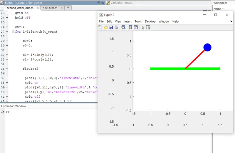
Error 1: I have used the formula y1=1*cos(y(i)) instead of y1=-1*cos(y(i))

Action: I have changed the formula.

OUTPUT:

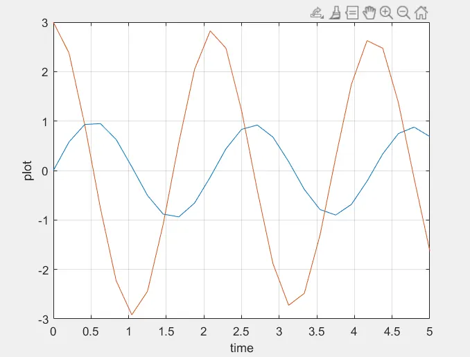
RESULT:

The Google drive link:

https://drive.google.com/file/d/1TtAsZOJWPHiR33HP2ziyc3mi1NpsvFbD/view?usp=sharing