Project 2 - Rankine cycle Simulator
AIM:
- Create a Rankine Cycle Simulator code to calculate the state points of the Rankine Cycle (any type of your choice) based on user inputs.
- Then, plot the corresponding T-s and h-s plots for the given set of inputs.
RANKINE CYCLE:
- The Rankine cycle is an idealized thermodynamic cycle describing the process by which certain heat engines, such as steam turbines or reciprocating steam engines, allow mechanical work to be extracted from a fluid as it moves between a heat source and heat sink.
-
Rankine cycle, in heat engines, ideal cyclical sequence of changes of pressure and temperature of a fluid, such as water, used in an engine, such as a steam engine. It is used as a thermodynamic standard for rating the performance of steam power plants.
- Process (1-2) : Isentropic compression
- Process (2-3) : Constant pressure heat addition in boiler
- Process (3-4) : Isentropic expansion
- Process (4-1) : Constant pressure heat rejection in condenser
Formula,
- WPump = H2 – H1
- Qadd = H3 – H2
- WTurbine = H4 – H3
- Qre = H4 – H1
- Wnet = WTurbine – WPump
- WR + BWR = 1
- WR (Work ratio) = Wnet/WTurbine
- BWR (Back work ratio) = WPump/WTurbine
- η (Thermal Effeciency) = Wnet/Qadd
- HR (Heat ratio) = 1/η
- SSC (Specific Steam ratio) = 1/Wnet
MAIN PROGRAM:
close all
clear all
clc

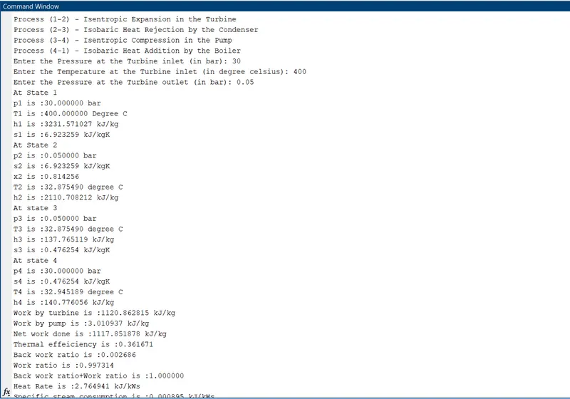
fprintf('Process (1-2) - Isentropic Expansion in the Turbine \n');
fprintf('Process (2-3) - Isobaric Heat Rejection by the Condenser \n');
fprintf('Process (3-4) - Isentropic Compression in the Pump \n');
fprintf('Process (4-1) - Isobaric Heat Addition by the Boiler \n');

p1=input('Enter the Pressure at the Turbine inlet (in bar): ');
T1=input('Enter the Temperature at the Turbine inlet (in degree celsius): ');
p2=input('Enter the Pressure at the Turbine outlet (in bar): ');

%At Point 1
hg_1=XSteam('hV_p',p1);
sg_1=XSteam('sV_p',p1);
Tsat_P1=XSteam('Tsat_p',p1);
Cp1_L=XSteam('CpL_p',p1);

%At Point 2
hg_2=XSteam('hV_p',p2);
sg_2=XSteam('sV_p',p2);
Tsat_P2=XSteam('Tsat_p',p2);
Cp2_V=XSteam('CpV_p',p2);

%At Point 3
hf_3=XSteam('hL_p',p2);
sf_3=XSteam('sL_p',p2);

%At Point 4
hf_4=XSteam('hL_p',p1);
sf_4=XSteam('sL_p',p1);

%State Vaariable at Point 1
fprintf('At State 1 \n');
fprintf('p1 is :%f bar \n',p1);
fprintf('T1 is :%f Degree C \n',p1);

h1=XSteam('h_pT',p1,T1);
fprintf('h1 is :%f kJ/kg \n',h1);

s1=XSteam('s_pT',p1,T1);
fprintf('s1 is :%f kJ/kgK \n',s1);

%State Vaariable at Point 2
fprintf('At State 2 \n');
fprintf('p2 is :%f bar \n',p2);

s2=s1;
fprintf('s2 is :%f kJ/kgK \n',s2);

if(s2<=sg_2)
    x2=(s2-sf_3)/(sg_2-sf_3);
else
    x2=1;
end
fprintf('x2 is :%f \n',x2);

if(x2<1)
    T2=Tsat_P2;
else
    T2=(Tsat_P2+273.15)*exp(s2-sg_2)/(Cp2_V);
    T2=T2-273.15;
end
fprintf('T2 is :%f degree C \n',T2);

if(x2<1)
    h2=hf_3+x2*(hg_2-hf_3);
else
    h2=XSteam('h_pT',p2,T2);
end
fprintf('h2 is :%f kJ/kg \n',h2);

fprintf('At state 3 \n')
p3=p2;
fprintf('p3 is :%f bar \n',p3);

V3=XSteam('vL_p',p3);

T3=Tsat_P2;
fprintf('T3 is :%f degree C \n',T3);

h3=hf_3;
fprintf('h3 is :%f kJ/kg \n',h3);

s3=sf_3;
fprintf('s3 is :%f kJ/kgK \n',s3);

fprintf('At state 4 \n')
p4=p1;
fprintf('p4 is :%f bar \n',p4);

s4=s3;
fprintf('s4 is :%f kJ/kgK \n',s4);

T4=XSteam('T_ps',p4,s4);
fprintf('T4 is :%f degree C \n',T4);

W_p=V3*(p4-p3)*100;
h4=W_p+h3;
fprintf('h4 is :%f kJ/kg \n',h4)

W_T=h1-h2;
fprintf('Work by turbine is :%f kJ/kg \n',W_T)
fprintf('Work by pump is :%f kJ/kg \n',W_p)

Wnet=W_T-W_p;
fprintf('Net work done is :%f kJ/kg \n',Wnet)

Qin=h1-h4;

eff_thermal=Wnet/Qin;
fprintf('Thermal effeiciency is :%f \n',eff_thermal);

b_w_r=(W_p/W_T);
fprintf('Back work ratio is :%f \n',b_w_r);
w_r=(Wnet/W_T);
fprintf('Work ratio is :%f \n',w_r);
fprintf('Back work ratio+Work ratio is :%f \n',(b_w_r+w_r));

H_R=(1/eff_thermal);
fprintf('Heat Rate is :%f kJ/kWs \n',H_R);
ssc=(1/Wnet);
fprintf('Specific steam consumption is :%f kJ/kWs \n',ssc');

temperature=linspace(0,T1,5000);
for i=1:length(temperature)
    H_l(i)=XSteam('hL_T',temperature(i));
    H_v(i)=XSteam('hV_T',temperature(i));
    S_l(i)=XSteam('sL_T',temperature(i));
    S_v(i)=XSteam('sV_T',temperature(i));
end

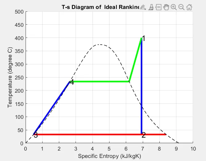
figure(1)
hold on

plot([s1 s2],[T1 T2],'color','blue','linewidth',3)
plot([s2 sg_2],[T2 Tsat_P2],'color','green','linewidth',3)
plot([sg_2 s3],[Tsat_P2 T3],'color','red','linewidth',3)
plot([s3 s4],[T3 T4],'color','green','linewidth',3)
plot([s4 sf_4],[T4 Tsat_P1],'color','blue','linewidth',3)
plot([sf_4 sg_1],[Tsat_P1 Tsat_P1],'color','green','linewidth',3)
plot([sg_1 s1],[Tsat_P1 T1],'color','green','linewidth',3)

text(s1,T1,'1','Fontsize',15)
text(s2,T2,'2','Fontsize',15)
text(s3,T3,'3','Fontsize',15)
text(sf_4,Tsat_P1,'4','Fontsize',15)

plot(S_l,temperature,'color','black','linestyle','--','linewidth',1)
plot(S_v,temperature,'color','black','linestyle','--','linewidth',1)

axis([0 10 0 500])
title('T-s Diagram of  Ideal Rankine Cycle')
ylabel('Temperature (degree C)')
xlabel('Specific Entropy (kJ/kgK)')
grid on

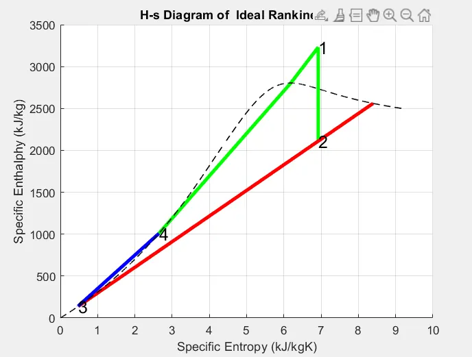
figure(2)
hold on

plot([s1 s2],[h1 h2],'color','green','linewidth',3)
plot([s2 sg_2],[h2 hg_2],'color','red','linewidth',3)
plot([sg_2 s3],[hg_2 h3],'color','red','linewidth',3)
plot([s3 s4],[h3 h4],'color','blue','linewidth',3)
plot([s4 sf_4],[h4 hf_4],'color','blue','linewidth',3)
plot([sf_4 sg_1],[hf_4 hg_1],'color','green','linewidth',3)
plot([sg_1 s1],[hg_1 h1],'color','green','linewidth',3)

text(s1,h1,'1','Fontsize',15)
text(s2,h2,'2','Fontsize',15)
text(s3,h3,'3','Fontsize',15)
text(sf_4,hf_4,'4','Fontsize',15)

plot(S_l,H_l,'color','black','linestyle','--','linewidth',1)
plot(S_v,H_v,'color','black','linestyle','--','linewidth',1)

title('H-s Diagram of  Ideal Rankine Cycle')
ylabel('Specific Enthalphy (kJ/kg)')
xlabel('Specific Entropy (kJ/kgK)')
grid on
EXPLANATION:
1.Describing the process of the rankine cycle stages
fprintf('Process (1-2) - Isentropic Expansion in the Turbine \n');
fprintf('Process (2-3) - Isobaric Heat Rejection by the Condenser \n');
fprintf('Process (3-4) - Isentropic Compression in the Pump \n');
fprintf('Process (4-1) - Isobaric Heat Addition by the Boiler \n');
2.This is used to give the input of the state variable at point 1
p1=input('Enter the Pressure at the Turbine inlet (in bar): ');
T1=input('Enter the Temperature at the Turbine inlet (in degree celsius): ');
p2=input('Enter the Pressure at the Turbine outlet (in bar): ');
3.Then calculate the all the state variable at all point from the given data
%At Point 1
hg_1=XSteam('hV_p',p1);
sg_1=XSteam('sV_p',p1);
Tsat_P1=XSteam('Tsat_p',p1);
Cp1_L=XSteam('CpL_p',p1);
%At Point 2
hg_2=XSteam('hV_p',p2);
sg_2=XSteam('sV_p',p2);
Tsat_P2=XSteam('Tsat_p',p2);
Cp2_V=XSteam('CpV_p',p2);
%At Point 3
hf_3=XSteam('hL_p',p2);
sf_3=XSteam('sL_p',p2);
%At Point 4
hf_4=XSteam('hL_p',p1);
sf_4=XSteam('sL_p',p1);
%State Vaariable at Point 1
fprintf('At State 1 \n');
fprintf('p1 is :%f bar \n',p1);
fprintf('T1 is :%f Degree C \n',p1);
h1=XSteam('h_pT',p1,T1);
fprintf('h1 is :%f kJ/kg \n',h1);
s1=XSteam('s_pT',p1,T1);
fprintf('s1 is :%f kJ/kgK \n',s1);
%State Vaariable at Point 2
fprintf('At State 2 \n');
fprintf('p2 is :%f bar \n',p2);
s2=s1;
fprintf('s2 is :%f kJ/kgK \n',s2);
if(s2<=sg_2)
x2=(s2-sf_3)/(sg_2-sf_3);
else
x2=1;
end
fprintf('x2 is :%f \n',x2);
if(x2<1)
T2=Tsat_P2;
else
T2=(Tsat_P2+273.15)*exp(s2-sg_2)/(Cp2_V);
T2=T2-273.15;
end
fprintf('T2 is :%f degree C \n',T2);
if(x2<1)
h2=hf_3+x2*(hg_2-hf_3);
else
h2=XSteam('h_pT',p2,T2);
end
fprintf('h2 is :%f kJ/kg \n',h2);
fprintf('At state 3 \n')
p3=p2;
fprintf('p3 is :%f bar \n',p3);
V3=XSteam('vL_p',p3);
T3=Tsat_P2;
fprintf('T3 is :%f degree C \n',T3);
h3=hf_3;
fprintf('h3 is :%f kJ/kg \n',h3);
s3=sf_3;
fprintf('s3 is :%f kJ/kgK \n',s3);
fprintf('At state 4 \n')
p4=p1;
fprintf('p4 is :%f bar \n',p4);
s4=s3;
fprintf('s4 is :%f kJ/kgK \n',s4);
T4=XSteam('T_ps',p4,s4);
fprintf('T4 is :%f degree C \n',T4);
4.Then calulate the Net work done, work ratio,back work ratio,heat rate and specific steam rate,thermal effeciency
W_p=V3*(p4-p3)*100;
h4=W_p+h3;
fprintf('h4 is :%f kJ/kg \n',h4)
W_T=h1-h2;
fprintf('Work by turbine is :%f kJ/kg \n',W_T)
fprintf('Work by pump is :%f kJ/kg \n',W_p)
Wnet=W_T-W_p;
fprintf('Net work done is :%f kJ/kg \n',Wnet)
Qin=h1-h4;
eff_thermal=Wnet/Qin;
fprintf('Thermal effeiciency is :%f \n',eff_thermal);
b_w_r=(W_p/W_T);
fprintf('Back work ratio is :%f \n',b_w_r);
w_r=(Wnet/W_T);
fprintf('Work ratio is :%f \n',w_r);
fprintf('Back work ratio+Work ratio is :%f \n',(b_w_r+w_r));
H_R=(1/eff_thermal);
fprintf('Heat Rate is :%f kJ/kWs \n',H_R);
ssc=(1/Wnet);
fprintf('Specific steam consumption is :%f kJ/kWs \n',ssc');
temperature=linspace(0,T1,5000);
for i=1:length(temperature)
H_l(i)=XSteam('hL_T',temperature(i));
H_v(i)=XSteam('hV_T',temperature(i));
S_l(i)=XSteam('sL_T',temperature(i));
S_v(i)=XSteam('sV_T',temperature(i));
end
5.Then plot a graph to plot H-s and T-s diagram
figure(1)
hold on
plot([s1 s2],[T1 T2],'color','blue','linewidth',3)
plot([s2 sg_2],[T2 Tsat_P2],'color','green','linewidth',3)
plot([sg_2 s3],[Tsat_P2 T3],'color','red','linewidth',3)
plot([s3 s4],[T3 T4],'color','green','linewidth',3)
plot([s4 sf_4],[T4 Tsat_P1],'color','blue','linewidth',3)
plot([sf_4 sg_1],[Tsat_P1 Tsat_P1],'color','green','linewidth',3)
plot([sg_1 s1],[Tsat_P1 T1],'color','green','linewidth',3)
text(s1,T1,'1','Fontsize',15)
text(s2,T2,'2','Fontsize',15)
text(s3,T3,'3','Fontsize',15)
text(sf_4,Tsat_P1,'4','Fontsize',15)
plot(S_l,temperature,'color','black','linestyle','--','linewidth',1)
plot(S_v,temperature,'color','black','linestyle','--','linewidth',1)
axis([0 10 0 500])
title('T-s Diagram of Ideal Rankine Cycle')
ylabel('Temperature (degree C)')
xlabel('Specific Entropy (kJ/kgK)')
grid on
figure(2)
hold on
plot([s1 s2],[h1 h2],'color','green','linewidth',3)
plot([s2 sg_2],[h2 hg_2],'color','red','linewidth',3)
plot([sg_2 s3],[hg_2 h3],'color','red','linewidth',3)
plot([s3 s4],[h3 h4],'color','blue','linewidth',3)
plot([s4 sf_4],[h4 hf_4],'color','blue','linewidth',3)
plot([sf_4 sg_1],[hf_4 hg_1],'color','green','linewidth',3)
plot([sg_1 s1],[hg_1 h1],'color','green','linewidth',3)
text(s1,h1,'1','Fontsize',15)
text(s2,h2,'2','Fontsize',15)
text(s3,h3,'3','Fontsize',15)
text(sf_4,hf_4,'4','Fontsize',15)
plot(S_l,H_l,'color','black','linestyle','--','linewidth',1)
plot(S_v,H_v,'color','black','linestyle','--','linewidth',1)
title('H-s Diagram of Ideal Rankine Cycle')
ylabel('Specific Enthalphy (kJ/kg)')
xlabel('Specific Entropy (kJ/kgK)')
grid on
ERRORS FACED:

ERROR : For the line breaking command instead of '\n' I have typed '/n'
ACTION : Error corrected.
OUTPUT:
1. T-s diagram of rankine cycle
2. H-s diagram of rankine cycle