Week 4.1 - Genetic Algorithm
What is Genetic Algorithm (GA)?
Genetic algorithm or GA is basically an optimization technique used to modify the quality of a particular species to fitter version of its original self. This technique follows the theory of Evolution proposed by Charles Darwin, which states that after a particular population is being initiated selection of most favourable among them is done after which several processes like crossover, mutation and then again selection of best population is done. GA runs this till a desired result is obtained.
Phases of Genetic Algorithm:
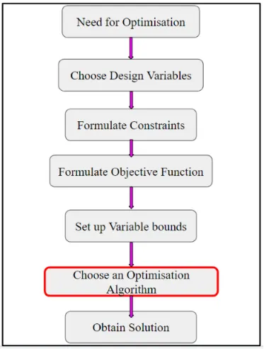
- Initiation of population
During this step we calculate the fitness of each individual member and this fitness calculation forms the pillar of next population which will be fitter and this step gives an idea about how the population is scattering about given input values.
- Fitness function
It is that function which we have to optimize using this population. Its optimization is done with next generation of population which was generated based on the fitness value of each member produced by the code.
- Selection of fittest
In this step, we find the fittest solution which can be used to produce the next generation of population and pass on their best genes. Main objective for this step is to find the region where there is a high chance of getting our outcome.
- Reproduction
Offspring generation happens in 2 ways
- Crossover
In this mating of parents is done at any random points which gives the offspring. This crossover is done in 3 different ways:
- Single point crossover - parents mating is done at a single point and off spring is produced
- Two - point crossover – parents mating happens either randomly or selectively at two points among the member.
- Uniform crossover – Each bit is chosen from each parent having equal probability.
- Mutation – Here a random bit among the member is flipped to produce the new diversity of species and fitter species. Mutation happens among genes with low random probability.
SYNTAX OF GA IN MATLAB
- x = ga(fun,nvars)
- x = ga(fun,nvars,A,b) - Here, A and b are subjected to the linear inequalities and related to each other by equation A * x <
- x = ga(fun,nvars,A,b,Aeq,beq) - In case of linear equalities 2 more variable matrices are introduced Aeq and beq which are related as Aeq * x < beq and in place of A and b ‘ [ ] ‘ will come.
- x = ga(fun,nvars,A,b,Aeq,beq,lb,ub) - To constrain the objective function we have to set the limits which are lower boundary (‘ lb ‘) and upper boundary (‘ ub ‘) to narrow down the search for desired results.
- x = ga(fun,nvars,A,b,Aeq,beq,lb,ub,nonlcon) – to constraint the function without limits we can introduce non-linear constraint in ‘ nonlcon ‘ which takes the output value of ‘ x ‘ to calculate that non linear constraint.
- x = ga(fun,nvars,A,b,Aeq,beq,lb,ub,nonlcon,options) – to modify the parameters involved in optimization ‘options ‘ is used. This is created using the command ‘optimoptions ‘.
- x = ga(fun,nvars,A,b,Aeq,beq,lb,ub,nonlcon,intcon) – here, ‘ intcon ‘ is used as an integer constraint to take it as output value and return ‘ x ‘ values based on that.
- x = ga(fun,nvars,A,b,Aeq,beq,lb,ub,nonlcon,intcon,options) – this is the full scale form of GA syntax.
- x = ga(problem)
In all the various syntax, ‘ x ’ represent the local (constrained or unconstrained) minimum of the objective function, ‘ nvars ‘ represent number of variables in objective function.
- [x,fval] = ga(___)
- [x,fval,exitflag,output] = ga(___) – here, ‘exitflag’ returns the integer value due to which the algorithm terminated and ‘ output ‘ returns the output from each generation and other performance values of algorithm.
- [x,fval,exitflag,output,population,scores] = ga(___) – here, ‘population’ returns the final population and ‘scores’ return value of score for the members of corresponding final population.
In above syntax, ‘ x ‘ returns minimum of the function and ‘ fval ‘ returns the value of fitness function at ‘ x ‘.
1. Code for Stalagmite function with an screenshot of original function
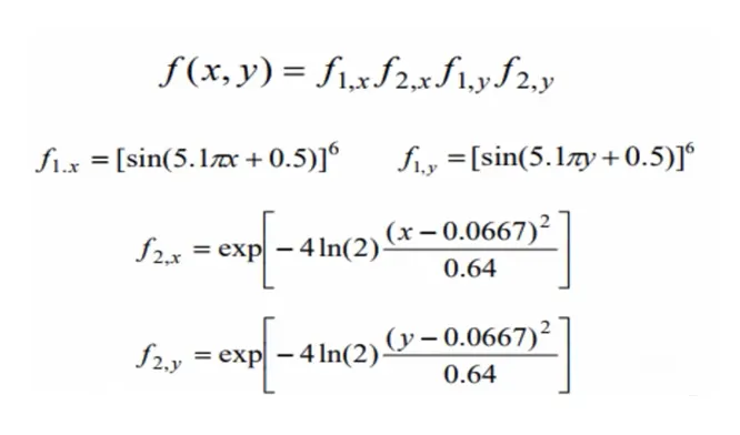
function [f] = stalagmite(input_vectors)

x=input_vectors(1);
y=input_vectors(2);
f1_x =(sin((5.1*pi*x)+0.5)).^6;
f1_y =(sin((5.1*pi*y)+0.5)).^6;
t1 = ((x-0.0667).^2)/0.64;
f2_x = exp(-4*log(2)*t1);
t2 = ((y-0.0667).^2)/0.64;
f2_y = exp(-4*log(2)*t2);

f = -(f1_x.*f1_y.*f2_x.*f2_y);

end
Above stalagmite function is coded separately that is thefunction is defined. and in this the output function 'f' is given as -ve sign to get the maxima of the function.
Now, after this, we can proceed for objective coding.
clc
clear all
close all

%inputs for function

x = linspace(0,0.6,150);
y = linspace(0,0.6,150);

[xx,yy] = meshgrid(x,y);

% evaluate the fitness function

num_cases = 50; % number of iterations
for i= 1:length(xx)
    for j = 1:length(yy)
        input_vectors(1) = xx(i,j);
        input_vectors(2) = yy(i,j);
        f(i,j) = stalagmite(input_vectors);    % function evaluation for each value of input variables
    end
end

% Study 1 to generate next offspring
tic
for i = 1:num_cases
    [inputs,fopt(i)] = ga(@stalagmite, 2);    % GA syntax with no restrictions (open search)
    xopt(i) = inputs(1);
    yopt(i) = inputs(2);
end
study1_time = toc      % gives the output of elapsed time for study 1

figure(1)
% plot 3-D graph for fitness against x and y values
subplot(2,1,1)
hold on
surfc(x,y,f)
shading interp
plot3(xopt,yopt,fopt,'Marker','o','MarkerFaceColor','r','markersize',4);
xlabel('X - axis');
ylabel('Y - axis');
subplot(2,1,2)
plot(fopt);
xlabel('Number of iterations');
ylabel('Function Maximum');

% Study 2 by applying boundary limits to narrow down the search
tic
for i = 1:num_cases
    [inputs,fopt(i)] = ga(@stalagmite, 2,[],[],[],[],[0;0],[0.6;0.6],[],[]);    % GA syntax with lower and upper bounds
    xopt(i) = inputs(1);
    yopt(i) = inputs(2);
end
study2_time = toc    % gives the output of elapsed time for study 2

figure(2)
% plot 3-D graph for optimized fitness against x and y values
subplot(2,1,1)
hold on
surfc(x,y,f)
shading interp

plot3(xopt,yopt,fopt,'Marker','o','MarkerFaceColor','r','markersize',4);
xlabel('X - axis');
ylabel('Y - axis');
subplot(2,1,2)
plot(fopt);
xlabel('Number of iterations');
ylabel('Function Maximum');

% Study 3 using optimoptions by varying population size
tic
options = optimoptions('ga');
options = optimoptions(options,"PopulationSize",300);
for i = 1:num_cases
    [inputs,fopt(i)] = ga(@stalagmite, 2,[],[],[],[],[0;0],[1;1],[],[],options);   % GA syntax with options and modified population size or iterations
    xopt(i) = inputs(1);
    yopt(i) = inputs(2);
end
study3_time = toc      % gives the output of elapsed time for study 3

figure(3)
% plot 3-D graph for fitness against x and y values
subplot(2,1,1)
hold on
surfc(x,y,f)
shading interp

plot3(xopt,yopt,fopt,'Marker','o','MarkerFaceColor','r','markersize',4);
xlabel('X - axis');
ylabel('Y - axis');
subplot(2,1,2)
plot(fopt);
axis([0 50 -1.1 -0.8])
xlabel('Number of iterations');
ylabel('Function maximum');
Explanation of abov code:
- Above code is generated to find the maximum value of the stalagmite function attached before the main code.
- The code starts from basic of ‘clc’, ‘clear all’ and ‘close all’ which clears text in command window, clears all variables from workspace and closes all figures, respectively.
- Then we introduce 2 variables ‘ x ‘ and ‘ y ‘ which contains values from 0 to 0.6. Using ‘meshgrid’ command we create a 2-D array for the input variables as ‘xx’ and ‘yy’.
- Next step is evaluating the stalagmite function using the ‘for’ loop. This gives us the idea about how the values are scattered. Stalagmite function is then evaluated using these 2-D arrays as ‘input vectors’
- After this first study is conducted to find the maximum of function using the genetic algorithm (‘ga’) without providing any limits, options and constraints. This code we make it run for 50 iterations using the ‘for’ loop. And record the values of function at each iteration in ‘fopt’ providing ‘xopt’ and ‘yopt’ as input and further, function ‘f’ values are plot against ‘x’ and ‘y’ values using ‘surfc’ command. We also plot the ‘fopt’ values against ‘xopt’ and ‘yopt’ as a 3-D plot using ‘plot3’ command. We use ‘subplot’ command to plot multiple plots in single figure window to understand 1 study at a time.
- Here we have also calculated the time it takes to do each study using the in-built tic’ and ‘toc’ command.
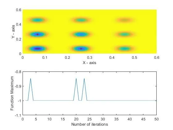
- After plotting the graph and using ‘ga’ syntax for 1st study wherein we provide 2 inputs in GA syntax which are ‘stalagmite’ function which needs to be optimized and number of variables used in this function i.e. ‘nvars’ as 2. As this part of code is made run it will provide different values of result each time we run the code. To overcome this fault, we need to provide the restrictions to the code which is done in study 2.
- In study 2, we restrict the code here by bounding the function between certain values, that is, by providing upper (‘ub’) and lower (‘lb’) boundaries to the syntax of ‘ga’. Providing this limits, code will narrow down its search to find the maximum of function.
- As we run the code for this section, through the graph we can understand that the results are now starting to converge and give us some constant results. Still there are some irregularities in the results to remove this ‘options’ is introduced.
- In study 3, we included one more part in ‘ga’ syntax called ‘options’. This is created using the function ‘optimoptions’. Using this command, we can optimize or modify some inputs which we already provided for the whole code and make it impact only for this part of ‘for’ loop in study 3. So, in this case we have modified the population size i.e. the number iterations to 300.
- Increasing the number of iterations will converge the final output rapidly and to know if in case the code is terminated we can give give one more out put in GA syntax as ‘exitflag’, it will give us an integer due to which this happened.
- For each case, we plot the same graph as in study 1 and provide ‘xlabel’ and ‘ylabel’ for better understanding.
Results:
1. Output graph for study 1 with plot for f values vs number of iterations.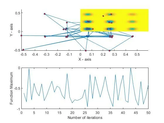
2. Output graph for study 2 with plot for f values vs number of iterations.
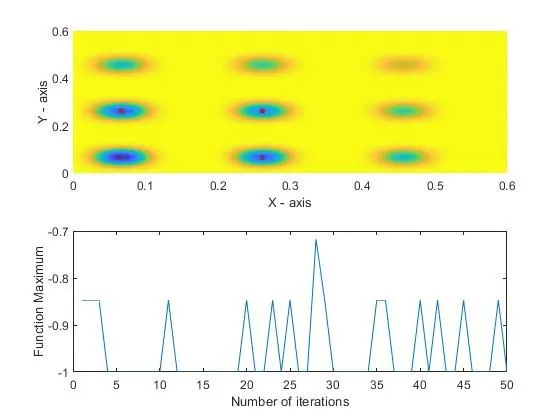
3. Output graph for study 3 with plot for f values vs number of iterations.
Links: