Week 3 - Solving second order ODEs
clc
clear all
close all

%Input for pendulum and damping motion
b=0.05;
g=9.81;
l=1;
m=1;
t_span = linspace(0,20,500);

%initial conditions
theta_0=[0;3];

%Solving the equation for pendulum
[t, results]=ode45(@(t,theta) ode_func(t,theta,b, g, l, m),t_span, theta_0);

%plotting graph of results
figure(1)
plot(results(:,1),'color','k')
hold on
plot(results(:,2),'color','r')
xlabel('Time');
ylabel('Amplitude');
legend('Angular displacement','Angular velocity')

figure(2)
% creating animation

ctr = 1;
for i = 1:length(t)
    O = [0 0];
    P = l*[sin(results(i,1)) -cos(results(i,1))];
    pend = plot([O(1) P(1)], [O(2) P(2)], 'LineWidth',2.5,'Color','r');
    hold on;
    ball = plot(P(1), P(2), 'o','MarkerSize',15,'MarkerEdgeColor','k','MarkerFaceColor','k');
    axis([-2 2 -2 2]);
    pause(0.02);
    M(ctr) = getframe(gcf);
    ctr=ctr+1;
      if i<ctr         %this loop is to delete previous graph so as to catch current graph for each frame
        delete(pend);
        delete(ball);
    end
end
% this part of code connects together all frames generated from above code
movie(M);
videofile = VideoWriter('Pendulum motion.avi','Uncompressed AVI');
videofile.FrameRate = 20;
open(videofile);
writeVideo(videofile,M);
close(videofile);
Above code is written to analyse the motion of pendulum and to understand the variation of angular displacement and angular velocity with respect to time.
The Damping motion of pendulum is understood using the following equation shown below.
`(d^2theta)/dt^2 + (b/m) * (d theta) / dt + (g/l) * sintheta = 0`
Here, ‘b’ is damping coefficient, ‘m’ is mass of bob, 'g' is acceleration due to gravity, ‘l’ is the length of pendulum.
This is a 2nd order ODE and to solve this we have to convert this into 2 first order derivatives. This conversion is shown in below code, which is written to create a function in MATLAB.
function dtheta_dt=ode_func(t, theta, b, g, l, m)
    theta1=theta(1);
    theta2=theta(2);
    dtheta1_dt=theta2;
    dtheta2_dt= -(b/m)*theta2 - (g/l)*sin(theta1);
    dtheta_dt = [dtheta1_dt; dtheta2_dt]
end
After this ‘ode_func’ is created, in the main code provide the input for ‘b’, ‘m’, ‘l’ and time span which is 20 seconds. We have to also provide the initial conditions of motion at time, t = 0. i.e. angular displacement = theta = 0 and angular velocity = ω = 3 rad/sec.
Then the MATLAB in-built function, ode45, is used to solve these derivatives. The output of this is matrix which gives values of angular velocity (ω) at each value of angular displacement (θ) for the number of points we required in the required time_span.
Next this result is plotted on a graph to show the variation of angular velocity with time and angular displacement with time.
Output 1: 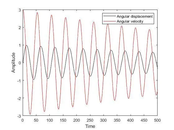
Output 2:
To create the animation of pendulum swinging we used the ‘movie’ command which connects the graph which is create after each for loop is completed. This for loop is working 500 times in 20 secs which gives us the animation of 20 secs.
In this ‘getframe(gcf) is mainly used to catch graph in each frame. And then connect it using ‘movie’ command.
Animation is provided at the below link on youtube.
https://youtu.be/urb6KzHHrH8