Week 4.1 - Genetic Algorithm

Aim:-

• To write a code in MATLAB to optimize the stalagmite function and find the function's global maxima.
• To explain the concept of genetic algorithm in your own words and also explain the syntax for ga in MATLAB in your report.
• To plot graphs for all 3 studies and F maximum vs no. of iterations.

Theory:-

Concept of Genetic Algorithm-

In 'ga', the minimum value of a function is calculated by default. So, to obtain the global maximum of a function, we invert the function whose global maximum we want to find, determine the smallest value of the inverted function, then subtract the negative of the minimum value to get the function's global maximum.

The Syntax for defining 'ga' in MATLAB-

Body of the content(Code):-

% Code in MATLAB to optimize the stalagmite function and to find the function's global maxima
clc 
clear all
close all

% Defining our search space 
% Independent varaibles
x = linspace(0,0.6,150);% x array
y = linspace(0,0.6,150);% y array

% Number of iterations
n = 50;

% Creating a 2 dimensional mesh
[xx,yy] = meshgrid(x,y);

% Evaluating the stalagmite function 
% Starting the loop
for i = 1:length(xx)
    for j = 1:length(yy)
        input_vector(1) = xx(i,j);
        input_vector(2) = yy(i,j);
        f(i,j) = stalagmite(input_vector);
    end
end

% Statistical Behaviour
% Study 1
tic
for i = 1:n
    [inputs,fopt(i)] = ga(@stalagmite,2);
    xopt(i) = inputs(1);
    yopt(i) = inputs(2);
end
study1_time = toc % Time taken for study

figure(1)
subplot(2,1,1)
hold on
surf(xx,yy,-f)% Creates a 3 dimensional surface
xlabel = ('X-axis');
ylabel = ('Y-axis');
title('Statistical Behaviour with Unbound inputs')
shading interp% Gives the appearance of a smoother surface
plot3(xopt,yopt,-fopt,'marker','o','markersize',5,'markerfacecolor','r')
subplot(2,1,2)
plot(-fopt)
xlabel = ('No. of Iterations');
ylabel = ('Function maximum');

% Study 2
tic
for i = 1:n
    [inputs,fopt(i)] = ga(@stalagmite,2,[],[],[],[],[0;0],[1,1]);
    xopt(i) = inputs(1);
    yopt(i) = inputs(2);
end
study2_time = toc % Time taken for study

figure(2)
subplot(2,1,1)
hold on
surf(xx,yy,-f)% Creates a 3 dimensional surface
xlabel = ('X-axis');
ylabel = ('Y-axis');
title('Statistical behaviour with upper and lower bounds')
shading interp% Gives the appearance of a smoother surface
plot3(xopt,yopt,-fopt,'marker','o','markersize',5,'markerfacecolor','r')
subplot(2,1,2)
plot(-fopt)
xlabel = ('No. of Iterations');
ylabel = ('Function maximum');

% Study 3
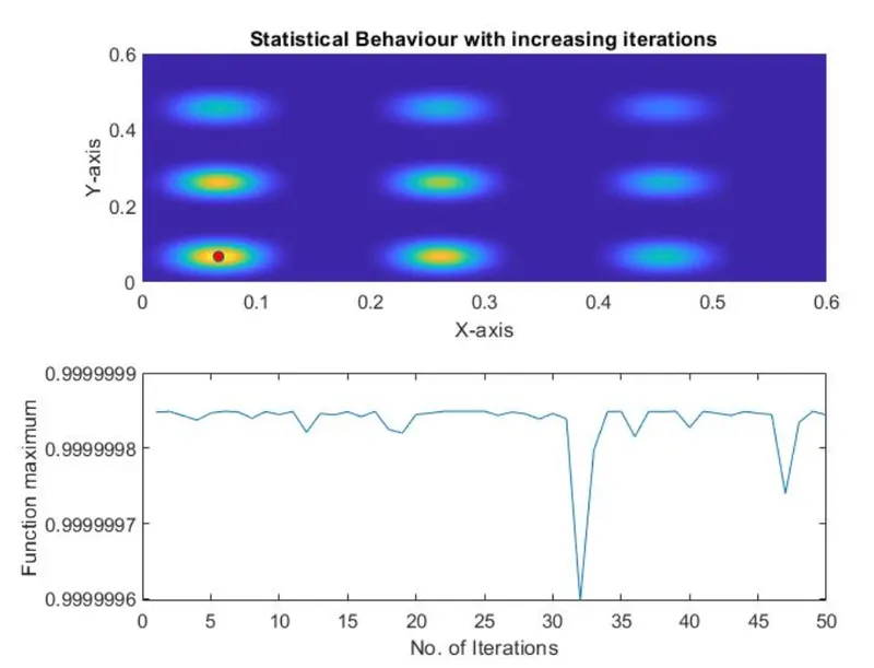
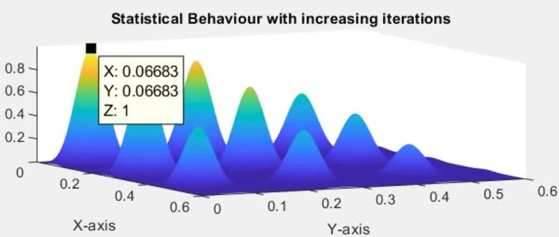
% Increasing the probability of the function by increasing the population size
options = optimoptions('ga');
options = optimoptions(options,'PopulationSize',400);

tic
for i = 1:n
    [inputs,fopt(i)] = ga(@stalagmite,2,[],[],[],[],[0;0],[1,1],[],[],options);
    xopt(i) = inputs(1);
    yopt(i) = inputs(2);
end
study3_time = toc % Time taken for study

figure(3)
subplot(2,1,1)
hold on
surf(xx,yy,-f)% Creates a 3 dimensional surface
xlabel = ('X-axis');
ylabel = ('Y-axis');
title('Statistical Behaviour with increasing iterations')
shading interp% Gives the appearance of a smoother surface
plot3(xopt,yopt,-fopt,'marker','o','markersize',5,'markerfacecolor','r')
subplot(2,1,2)
plot(-fopt)
xlabel = ('No. of Iterations');
ylabel = ('Function maximum');

Function Used:-

% Stalagmite Function
function [f] = stalagmite(input_vector)

a = input_vector(1);
b = input_vector(2);

f1 = (sin(((5.1)*pi*a)+(0.5)))^6;       % Term1
f2 = exp(-4*log(2)*((a-0.0667)^2)/0.64);% Term2
f3 = (sin(((5.1)*pi*b)+(0.5)))^6;       % Term3
f4 = exp(-4*log(2)*((b-0.0667)^2)/0.64);% Term4

[f] = -(f1*f2*f3*f4);% The function's negative sign will invert the stalagmite plot, resulting in the function's maxima

end

Explanation of code:-

1. Before starting the main code, I have used the commands. "clc" for clearing the command window, "clear all" for clearing all the previous variables, and "close all" for closing all the previous plots.

2. To begin, we'll create our own function to calculate the value of the objective function for various x and y values. We'll use the linspace command to do so. Using the meshgrid function, we now generate a matrix. Now we can use the values from the various matrices we've built as inputs to the function we've created by calling it. This allows us to determine the function's value at various x and y values. Now that we have the function's value at various values, we must compute the maximum value, which can be done with the help of the built-in function 'ga'. So for our first study, we will use the for loop and iterate it 50 times.

3. To evaluate the stalagmite function, for loop is used where 'i' is initialized and for every value of 'i' another for loop is used to initialize 'j'.

4. The 'xx' and 'yy' input vector values are defined, as well as the stalagmite function for these input vectors. This will result in a simple stalagmite function, which we can plot separately if necessary.

5. Following the preparation of the function's inputs, the following stage is to obtain the results for three situations of the genetic algorithm. In the first case or study, the function's maximum value is obtained with no limitations, bounds, or limits. This is accomplished via a for loop in which we utilize the 'ga' syntax to provide values for inputs and the best maximum value. In ga syntax, the stalagmite function is called, and the amount of variables 'nvars' is 2.

6. The 'tic' and 'toc' commands are used before and after the loop, respectively, to find out how long it takes to solve the loop for 50 iterations.

Errors faced:-

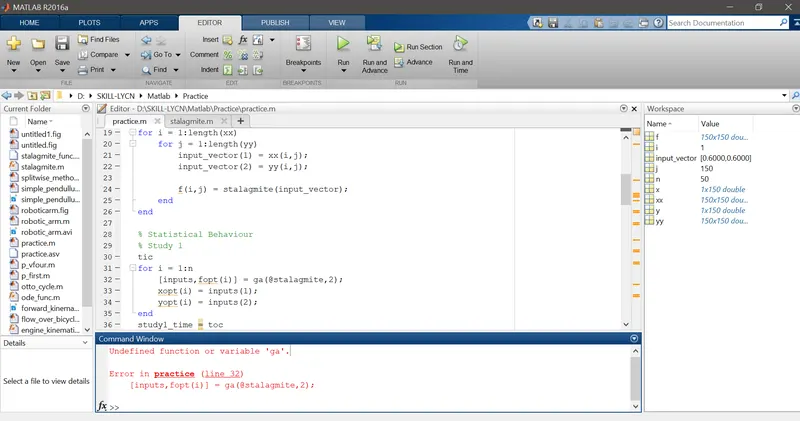
Previously I have not installed the package for global optimization, that's why it is continuously giving this error - Undefined function or variable 'ga'.

Conclusion and Final results:-

Study 1 -

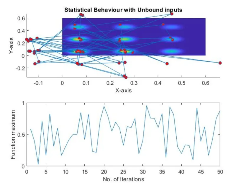
The random sampling of the genetic algorithm provides a new optimum value for the function every time the code is executed, as shown in this plot. This, however, is consistent with the concept of a Genetic Algorithm. A vast number of red dots represent the values of x and y coordinates, which change with each iteration.

Study 2 -

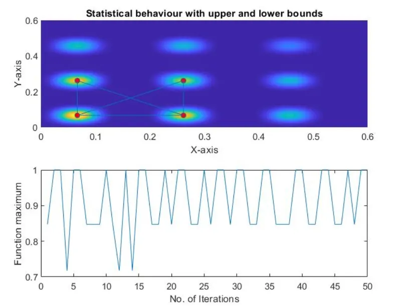
The results of this plot demonstrate the convergence of x and y values. In comparison to the previous plot, there are less red dots. This is the effect of giving the function upper and lower boundaries.

Study 3 -