Week 3 - Solving second order ODEs

Aim:-

- To write a program that solves the simple pendulum ODE.

- To animate the motion of the pendulum.

Governing Equations:-

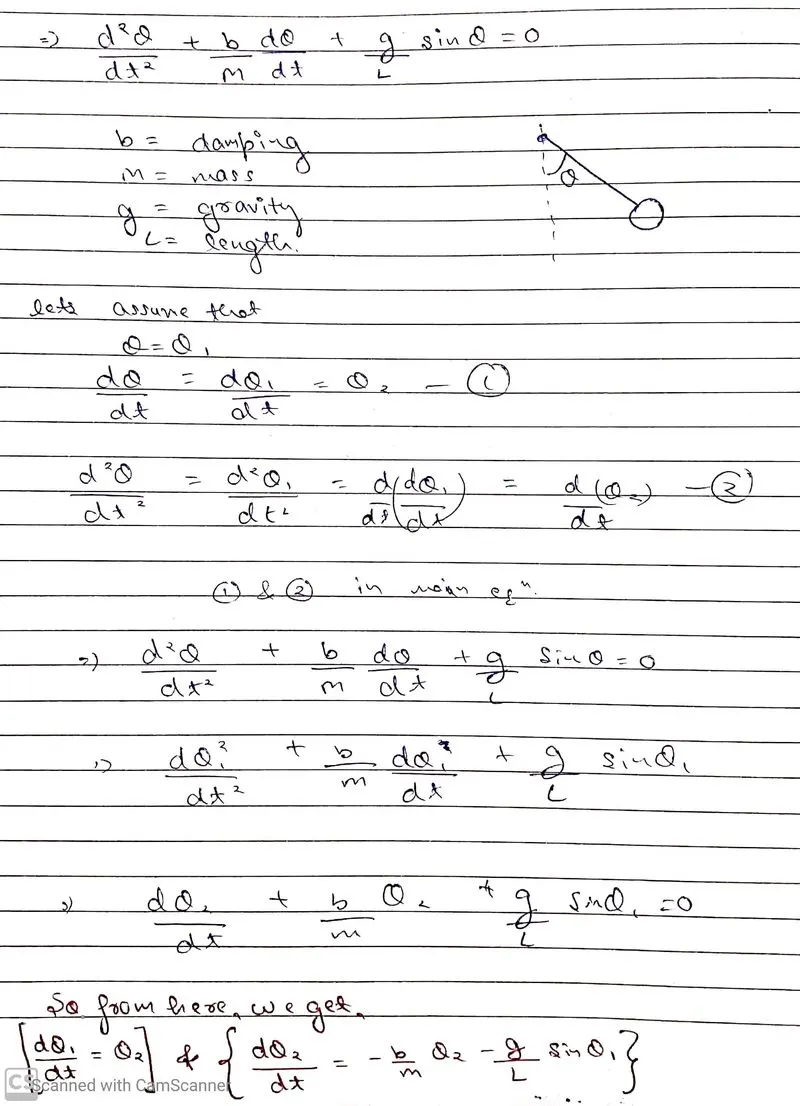
As shown in the figure, after equating all the equations we get two simple equations by which we can solve the ODE.

Body of the content(Code):-

%A program that solves the simple pendulum ODE
clc
clear all 
close all

%Inputs 
b=0.05;
g=9.81;
l=1;
m=1;

%Initial condition
theta_0 = [0;3];

%Time points
t_span = linspace(0,10,100);

%Solve ODE
[t, results] = ode45(@(t,theta) ode_func(t,theta,b,g,l,m),t_span,theta_0);

%Plotting the curves
A=plot(t,results(:,1));
hold on
B=plot(t,results(:,2));
title('Simple Pendulum');
xlabel('Position(in radians)');
ylabel('Plots');
legend([A,B],'Displacement','Angular Velocity');
grid on

Function Used:-

%Function for solving ODE
function [dtheta_dt] = ode_func(t,theta,b,g,L,m)
theta1 = theta(1);
theta2 = theta(2);

dtheta1_dt = theta2;
dtheta2_dt = -(b/m)*theta2-(g/L)*sin(theta1);


dtheta_dt = [dtheta1_dt;dtheta2_dt];
end

Simulation Code:-

%Simulation Of Simple Pendulum

count=1;
for i=1:length(results(:,1))

    x0 = 0;
    y0 = 0;

    x1 = L*sin(results(i,1));
    y1 = -L*cos(results(i,1));
    
    %Plotting the Simple Pendulum
    plot([-0.5,0.5],[0,0],'linewidth',5,'color','k');%Ceiling 
    grid on 
    hold on
    plot([x0 x1],[y0 y1],'linewidth',2,'color','b');%Rope
    plot(x1,y1,'o','MarkerSize',20,'markerfacecolor', 'r');%Ball
    axis([-1.5 1.5 -1.5 0.5]);
    title('Simple Pendulum');
    xlabel('X-axis');
    ylabel('Y-axis');
    pause(0.02);
    hold off
    M(count)=getframe(gcf);
    count = count+1;
end

%Making the movie
movie(M);
videofile=VideoWriter('simple_pendullum.avi','Uncompressed AVI');
open(videofile);
writeVideo(videofile,M);
close(videofile);

Explanation of code:-

1. Before starting the main code, I have used the commands. "clc" for clearing the command window, "clear all" for clearing all the previous variables, "close all" for closing all the previous plots.

2. Then I have given the inputs. As b=damping coefficient, g = gravity in m/s2, L = length of the pendulum in m, m = mass of the ball in kg.

3. Then I have to give the initial condition as angular displacement=0 and angular velocity=3 rad/sec at time t=0. So I have created a column matrix as "theta_0 = [0;3]".

4. Then for a time interval(t_span) I used "linspace" command, starting with 0 sec, ending with 10 sec and having 100 intervals including them.

5. For solving ODE I used a function namely ode_func. By calling it with the inputs t, theta, b, g, L,m. According to the above figure shown, I have assign the theta(1) value to theta1 and theta(2) value to theta2. Then finally we got the two eqations, which I writted in the program.

6. Then I have assinged these values to a column matrix "dtheta_dt". Finally ending this function with the help of "end" command.

7. Now coming to the main program, I used "ode45" funtion of MATLAB to solve the ODE. Then finally I stored the these outputs to [t, results].

8. Then for plotting the curves I have used "plot" command. First for displacement plot, assigned to A and then for angular velocity, assigned to B.

9. Then I applied title, xlabel, ylabel, legend and grid with respective commands.

10. Here we completed a program that solves and the simple pendulum ODE.

i. For simulation, I added a counter variable as "count" for counting the total number of frames required for animation making.

ii. So now the main logic comes, basically for each row of "results" has 100 dirrefert values. So I used for loop for that. First we have to define a origin, where the string is hinged, so I take the origin as (x0,y0)=(0,0). Then for the ball position, we can find its coordinates(x1,y1) by using tignometry. x1 = L*sin(Q) , y1 = -L*cos(Q).

iii. Then I plotted the line as a ceiling, with the help of plot command, and applying hold abd grid commande with respective commands. After that I plotted the rope with thw "plot" command. And then finally the ball.

iv. Then I have given the axis for the plot. with "axis" command. Then I have added the title, and x & y labels for the plot.

v. Now we are ready for a plot. But to see it nicely, we have to give a pause to it with a "pause" command. And after that a "hold off" command to hold the plot.

vi. Now for the animation of the plot, I have used "getframe" command to collect the current frame and stored it in an array as "M". Now after getting the frame, I have given an increment of +1 in "count" so that it can run again and collect the next frame.

vii. After this I have closed the for loop with the "end" command.

viii. Now for making the movie, I named it as "simple_pendulum.avi", to make an uncompressed AVI file. Now opening this file with "open" command and then read and write all the frames collected in "M". And then closed the file.

Errors faced:-

Previously I didn't use the "hold off" command after the "plot" command in simulation code.

%Simulation Of Simple Pendulum

count=1;
for i=1:length(results(:,1))

    x0 = 0;
    y0 = 0;

    x1 = L*sin(results(i,1));
    y1 = -L*cos(results(i,1));
    
    %Plotting the Simple Pendulum
    plot([-0.5,0.5],[0,0],'linewidth',5,'color','k');%Ceiling 
    grid on 
    hold on
    plot([x0 x1],[y0 y1],'linewidth',2,'color','b');%Rope
    plot(x1,y1,'o','MarkerSize',20,'markerfacecolor', 'r');%Ball
    axis([-1.5 1.5 -1.5 0.5]);
    title('Simple Pendulum');
    pause(0.02);
    M(count)=getframe(gcf);
    count = count+1;
end

%Making the movie
movie(M);
videofile=VideoWriter('simple_pendullum.avi','Uncompressed AVI');
open(videofile);
writeVideo(videofile,M);
close(videofile);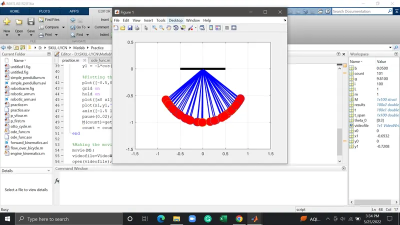

Conclusion and final results:-

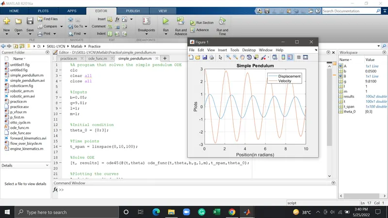
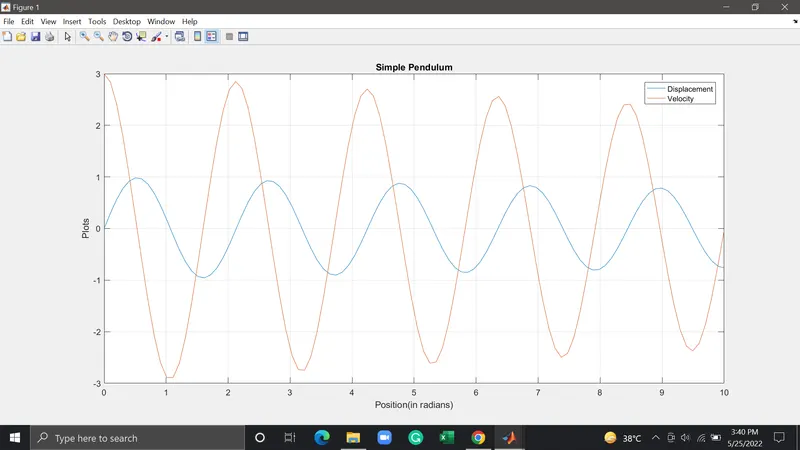
Simulation:-

Youtube link - https://youtu.be/eGWxfVAHAjI