Project 2 - Rankine cycle Simulator
Aim:-
Create a Rankine Cycle Simulator using OCTAVE/MATLAB.
Objective:-
- To calculate the state points of the Rankine Cycle based on user inputs.
- To plot the corresponding T-s and h-s plots for the given set of inputs.
Theory:-
The Rankine cycle is a heat-to-mechanical energy conversion mechanism utilised in power plants. Water is generally used as a working fluid. External fuel is used to transform water into steam, which expands through the turbine and creates work in this cycle. The pump and turbine in an ideal Rankine cycle would be isentropic, maximising net work output while generating no entropy. We're also assuming that water to steam and steam to water conversion takes place at constant pressure.
Because fluid friction produces irreversibility and heat loss to the surrounding causes a loss of work production, the actual Rankine cycle differs from the ideal Rankine cycle. Pressure declines between the boiler and condenser, causing steam to leave the boiler at a lower pressure.
Reheat and regeneration processes can be used to alter the Rankine cycle. Heat is exchanged between the working fluid and compressed fluid before heat is added in the Regenerative cycle, which eliminates moisture transported by steam at the last step of the expansion process, increasing the cycle's thermal efficiency. The regenerative cycle reduces the amount of heat provided to the boiler while increasing its efficiency.
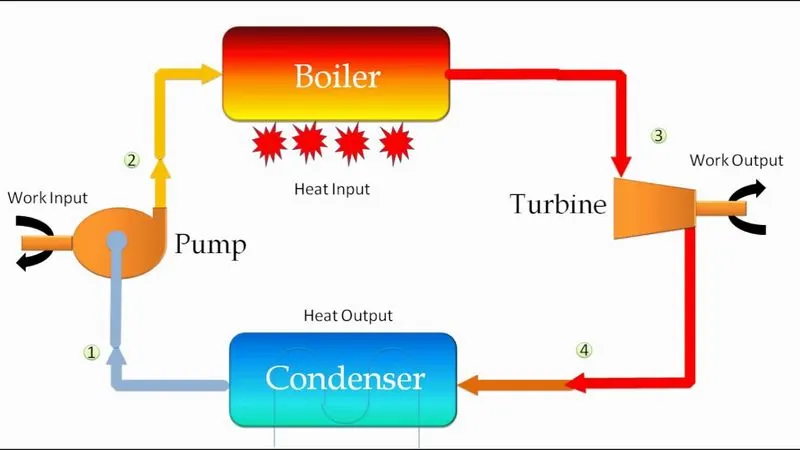
The Rankine cycle is made up of four steps:-
1. Isentropic expansion - Steam enters the turbine and is expanded by the turbine, lowering pressure and temperature. Electricity is generated by the turbine.
2. Constant pressure heat rejection - Wet steam rejects heat into the condenser, where it changes phase and becomes saturated liquid.
3. Isentropic compression - Water is pumped isentropically from low to high pressure, and the pump requires some input to do so.
4. Constant pressure heat addition - Water enters the boiler and is heated until it changes phase to dry saturated vapor. Because the process is carried out under constant pressure and heat is added to the water, it is referred to as constant pressure heat addition.
Governing Equations:-
Some basic variables - (P for Pressure, T for Temperature, H for Enthalpy, S for Entropy, W for Work)
H1 = enthalpy at the turbine inlet
H2 = enthalpy at the turbine outlet
H3 = enthalpy at pump inlet
H4 = enthalpy at the pump outlet
`w_t` = work done by the turbine
`w_p` = work taken by pump
Formulas:-
Heat addition(`Q_a`) = H1 - H4
Heat rejection(`Q_r`) = H2 - H3
Work done by turbine(`w_t`) = H1 - H2
Work taken by pump(`w_p`) = H4 - H3
Thermal efficiency(n) = `(w_t-w_p)/Q_a`
Net work output(`w_n`) = `w_t-w_p`
Back work ratio(BWR) = `w_p/w_t`
Body of the content(Code):-
% Rankine Cycle Simulator using MATLAB
clc
clear all
close all

% Displaying
disp('         Rankine Cycle Simulator')
fprintf('\n 1-2 is the Isentropic expansion')
fprintf('\n 2-3 is the Constant pressure heat rejection')
fprintf('\n 3-4 is the Isentropic compression')
fprintf('\n 4-1 is the Constant pressure heat addition')

% Stage-1 inputs
P1 = 30;% Given
T1 = 400;% Given
H1 = XSteam('h_pT',30,400);
S1 = XSteam('s_ph',30,H1);
fprintf('\n\n           Results')
fprintf('\n At state point 1')
fprintf('\n P1 is : %f bar',P1)
fprintf('\n T1 is : %f degree celcius',T1)
fprintf('\n H1 is : %f KJ/Kg',H1)
fprintf('\n S1 is : %f KJ/Kgk',S1)

% Stage-2 inputs
P2 = 0.05;% Given
S2 = S1;
T2 = XSteam('T_ps',0.05,6.1858);
sf2 = XSteam('sL_p',P2);
sg2 = XSteam('sV_p',P2);
hf2 = XSteam('hL_p',P2);
hg2 = XSteam('hV_p',P2);
x = ((S2 - sf2)/(sg2 - sf2));
H2 = hf2 + (x*(hg2 - hf2));
V2 = XSteam('v_ph',P2,H2);
fprintf('\n\n At state point 2')
fprintf('\n P2 is : %f bar',P2)
fprintf('\n T2 is : %f degree celcius',T2)
fprintf('\n H2 is : %f KJ/Kg',H2)
fprintf('\n S2 is : %f KJ/Kgk',S2)

% Stage-3 inputs
T3 = T2;
P3 = P2;
S3 = XSteam('sL_p',P3);
H3 = XSteam('hL_T',32.875);
V3 = XSteam('v_ph',P3,H3);
fprintf('\n\n At state point 3')
fprintf('\n P3 is : %f bar',P3)
fprintf('\n T3 is : %f degree celcius',T3)
fprintf('\n H3 is : %f KJ/Kg',H3)
fprintf('\n S3 is : %f KJ/Kgk',S3)

% Stage-4 inputs
S4 = S3;
V4 = V3;
P4 = P1;
H4 = XSteam('h_ps',P4,S4);
T4 = XSteam('T_hs',H4,S4);
fprintf('\n\n At state point 4')
fprintf('\n P4 is : %f bar',P4)
fprintf('\n T4 is : %f degree celcius',T4)
fprintf('\n H4 is : %f KJ/Kg',H4)
fprintf('\n S4 is : %f KJ/Kgk',S4)

% Stage-5 inputs
P5 = P4;
T5 = XSteam('Tsat_p',P5);
H5 = XSteam('hL_T',T5);
S5 = XSteam('sL_p',P5);
fprintf('\n\n At state point 5')
fprintf('\n P5 is : %f bar',P5)
fprintf('\n T5 is : %f degree celcius',T5)
fprintf('\n H5 is : %f KJ/Kg',H5)
fprintf('\n S5 is : %f KJ/Kgk',S5)

% Stage-6 inputs
T6 = T5;
P6 = XSteam('psat_T',T5);
S6 = XSteam('sV_T',T6);
H6 = XSteam('hV_T',T6);
fprintf('\n\n At state point 6')
fprintf('\n P6 is : %f bar',P6)
fprintf('\n T6 is : %f degree celcius',T6)
fprintf('\n H6 is : %f KJ/Kg',H6)
fprintf('\n S6 is : %f KJ/Kgk',S6)

% Variables on sturation lines are found using loops
t = linspace(0,400,1000);
for i = 1:length(t)
    s_line1(i) = XSteam('sL_T',t(i));
end
for j = 1:length(t)
    s_line2(j) = XSteam('sV_T',t(j));
end

for i = 1:length(t)
    h_line1(i) = XSteam('hL_T',t(i));
end
for j = 1:length(t)
    h_line2(j) = XSteam('hV_T',t(j));
end

% Calculation of Net Work output
W_turbine = H1 - H2;% Work done by turbine
W_pump = H4 - H3;% Work taken by pump
work = W_turbine - W_pump;% Net work output
Q_in = H1 - H4;% Heat addition
Q_out = H2 - H3;% Heat rejection

% Thermal efficiency of the turbine
n = work/Q_in;

% Net Work Output
W_n = W_turbine - W_pump;
fprintf('\n\n\n Net Work Output = %f',W_n)

% Back work ratio
BWR = W_pump/W_turbine;
fprintf('\n Back work Ratio = %f',BWR)

% Plotting T-S graph
figure(1)
hold on
plot([s_line1 s_line2],[t t])
plot([S1 S2 S3 S4 S5 S6 S1],[T1 T2 T3 T4 T5 T6 T1])
text(S1,T1,'1')
text(S2,T2,'2')
text(S3,T3,'3')
text(S4,T4,'4')
text(S5,T5,'5')
text(S6,T6,'6')
xlabel('Entropy(KJ/Kgk)')
ylabel('Temperature(k)')
title('Rankine Cycle(T-S Diagram)')
axis([0,10,0,500])
grid on

% Plotting H-S graph
figure(2)
hold on
plot([s_line1 s_line2],[h_line1 h_line2])
plot([S1 S2 S3 S4 S5 S6 S1],[H1 H2 H3 H4 H5 H6 H1])
text(S1,H1,'1')
text(S2,H2,'2')
text(S3,H3,'3')
text(S4,H4,'4')
text(S5,H5,'5')
text(S6,H6,'6')
xlabel('Entropy(KJ/Kgk)')
ylabel('Enthalpy(KJ/Kg)')
title('Rankine Cycle(H-S Diagram)')
axis([0,10,0,4000])
grid on
Explanation of code:-
Errors faced:-
No big error occurs, only some typing mistakes were there.
Conclusion and Final results:-
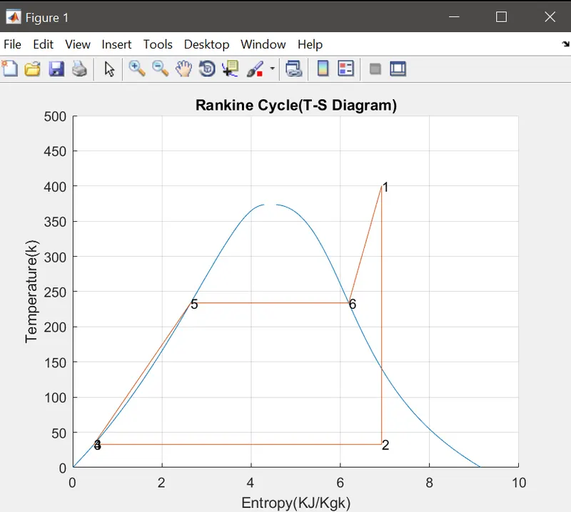
T-S Diagram
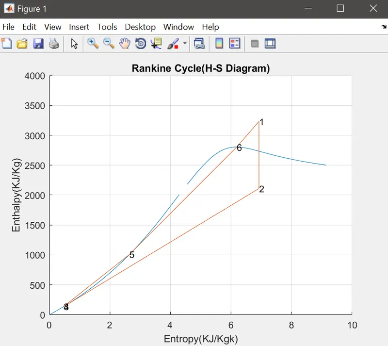
H-S Diagram
Command window, showing the outputs -
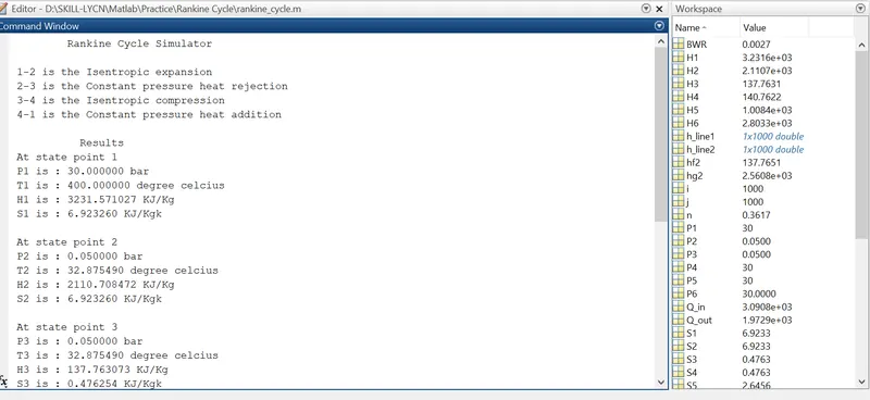
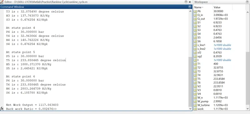
Net Work Output = 1117.863403
Back work Ratio = 0.002676
References:-
https://en.wikipedia.org/wiki/Rankine_cycle
https://in.mathworks.com/help/physmod/simscape/ug/rankine-cycle-steam-turbine.html