Week 4.1 - Genetic Algorithm

AIM: Write a code in MATLAB to optimize the stalagmite function and find the global maxima of the function.

OBJECTIVE: 1. Explain the concept of genetic algorithm and also explain the syntax for ga in MATLAB.

2. Plot graphs for all the 3 studies and for F maximum vs no. of iterations.

THEORY:

What is Genetic algorithms?

The genetic algorithm is a method for solving both constrained and unconstrained optimization problems that is based on natural selection, the process that drives biological evolution. The genetic algorithm repeatedly modifies a population of individual solutions. At each step, the genetic algorithm selects individuals from the current population to be parents and uses them to produce the children for the next generation.

Some basic concept and terminology used in GAs likes -

Optimization: It is the process of making the best or most effective use of a situation or resource.

It is used for finding the point that minimizes a function. More specifically:

• A local minimum of a function is a point where the function value is smaller than or equal to the value at nearby points, but possibly greater than at a distant point.
• A global minimum is a point where the function value is smaller than or equal to the value at all other feasible points.

Unconstrained means that the choice variable can take on any value - there are no restrictions.

Constrained means that the choice variable can only take on certain values within a larger range.

Constrained Optimization – It is the process of optimizing an objective function with respect to some variable in the presence of constraints on those variables.

Fitness function: The fitness function is the function you want to optimize. For standard optimization algorithms, this is known as the objective function. The toolbox software tries to find the minimum of the fitness function.

Write the fitness function as a file or anonymous function, and pass it as a function handle input argument to the main genetic algorithm function.

Fitness value: The fitness value of an individual is the value of the fitness function for that individual. Because the toolbox software finds the minimum of the fitness function, the best fitness value for a population is the smallest fitness value for any individual in the population.

Flow chart outlines of Genetic Algorithms

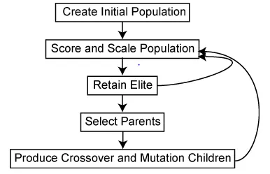
The genetic algorithm uses three main types of rules at each step to create the next generation from the current population:

• Selection rules select the individuals, called parents that contribute to the population at the next generation. The selection is generally stochastic, and can depend on the individuals' scores.
• Crossover rules combine two parents to form children for the next generation.
• Mutation rules apply random changes to individual parents to form children.

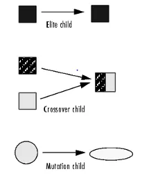
SYNTAX of GA - Find minimum of function using genetic algorithm. It is consists of inputs and output arguments.

x = ga(fun,nvars)

x = ga(fun,nvars,A,b)

x = ga(fun,nvars,A,b,Aeq,beq)

x = ga(fun,nvars,A,b,Aeq,beq,lb,ub)

x = ga(fun,nvars,A,b,Aeq,beq,lb,ub,nonlcon)

x = ga(fun,nvars,A,b,Aeq,beq,lb,ub,nonlcon,options)

x = ga(fun,nvars,A,b,Aeq,beq,lb,ub,nonlcon,intcon)

x = ga(fun,nvars,A,b,Aeq,beq,lb,ub,nonlcon,intcon,options)

x = ga(problem)

[x,fval] = ga(___)

[x,fval,exitflag,output] = ga(___)

[x,fval,exitflag,output,population,scores] = ga(___)

Input arguments

fun is objective function.

nvars is number of variables of fun.

A is real matrix of linear inequality constraints.

b is real vector of linear inequality constraints.

Aeq is real matrix of linear equality constraints.

beq is real vector of linear equality constraints.

lb is lower bound on x.

ub is upper bound on x.

nonlcon is nonlinear constraints.

Options created using optimoptions or an options structure.

intcon is integer variables.

Output arguments

x is solution, the best points that ga locate during its iterations.

fval is objective function value at solution i.e. x.

exitflag is reason that ga stopped.

output gives information about optimisation process.

population give final population.

scores give final score

Following are the condition or criteria for stopping the algorithm.

• MaxGenerations - Specifies the maximum number of iterations for the genetic algorithm to perform. The default is 100*numberOfVariables.
• MaxTime - The algorithms stop after running for an amount of time in seconds equal to MaxTime.
• MaxStallGenerations - The algorithm stop when the average relative change in the fitness function value over MaxStallGenerations is less then Function tolerance.
• MaxStallTime - The algorithm stop if there is no improvement in the objective function during an interval of time in seconds equal to MaxStallTime.
• FitnessLimit - The algorithm stops if the best fitness value is less than or equal to the value of FitnessLimit.
• ConstraintTolerance — The ConstraintTolerance is not used as stopping criterion. It is used to determine the feasibility with respect to nonlinear constraints. Also, max(sqrt(eps), ConstraintTolerance) determines feasibility with respect to linear constraints.

The algorithm stops as soon as any one of these conditions is met.

Stalagmite function:

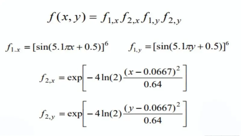
Stalagmite function is a mathematical function which generate several local and global maxima of the function with the help of equation.

The equation stalagmite function is given below:

Function code:

function f=stalagmite(input_vector)

x=input_vector(1);
y=input_vector(2);

f1_x=(sin(5.1*pi*x+0.5)).^6;
f1_y=(sin(5.1*pi*y+0.5)).^6;
f2_x=exp(-4.*log(2)*((x-0.0667).^2/0.64));
f2_y=exp(-4.*log(2)*((y-0.0667).^2/0.64));

f=-(f1_x*f1_y*f2_x*f2_y);
end

Note : To get global maxima of the function add negative sign with the function to inverse the result.

Main code:

clear all    % for clearing the stored data of workspace
close all    % for close the previous figures
clc          % for clear the data of command window

x=linspace(0,0.6,150);   % create a array of x variable.
y=linspace(0,0.6,150);   % create a array of y variable.


[X,Y]=meshgrid(x,y);     % create the martix X and Y of vector x and y 

% evaluating the stalagmite function
for i=1:length(X)
    for j=1:length(Y)
        input_vector(1)=X(i,j);
        input_vector(2)=Y(i,j);
         f(i,j)=stalagmite(input_vector);
    end
end

% Study case 1 - Statistical Behaviour
norm_counts=50;          % No. of iteration or generations preformed in ga.
% tic
for i=1:norm_counts
    [inputs1,fopt1(i)]=ga(@stalagmite,2);
    xopt1(i) = inputs1(1);
    yopt1(i) = inputs1(2);
end
t1=toc

figure(1)

subplot(2,1,1)     % divide area of plot into two half
surfc(X,Y,f)      % creating surface countour for mesh of X and Y with function output
shading interp
hold on            
% create a 3D plot for every optimal function at each iteration. 
plot3(xopt1,yopt1,fopt1,'marker','o','markersize',5,'markerfacecolor','r')  
title('Unbounded inputs')
xlabel('X value')
ylabel('Y value')

% create a plot of best or optimized function value at every iteration
subplot(2,1,2)     
plot(fopt1)
xlabel('No. of itertion')
ylabel('F Maximum')    % maximum function value at every iterations


% Study Case 2 - with lower and upper bounded

tic
for i=1:norm_counts
    [inputs2,fopt2(i)]=ga(@stalagmite,2,[],[],[],[],[0 0],[1 1]);
    xopt2(i) = inputs2(1);
    yopt2(i) = inputs2(2);
end
t2=toc

figure(2)

subplot(2,1,1)
surfc(X,Y,f)
shading interp
hold on
% create a 3D plot for every optimal function at each iteration.
plot3(xopt2,yopt2,fopt2,'marker','o','markersize',5,'markerfacecolor','r')
title('Bounded inputs')
xlabel('X value')
ylabel('Y value')

% create a plot of best or optimized function value at every iteration
subplot(2,1,2)
plot(fopt2)
xlabel('No. of iteration')
ylabel('F Maximum')    % maximum function value at every iterations

% case - 3 bounded inputs with increased polulation size default value (50) to 200
options = optimoptions('ga');  
options = optimoptions(options,'PopulationSize',200);

tic
for i=1:norm_counts
    [inputs3,fopt3(i)]=ga(@stalagmite,2,[],[],[],[],[0;0],[1;1],[],[],options);
    xopt3(i) = inputs3(1);
    yopt3(i) = inputs3(2);
end
t3=toc

figure(3)
subplot(2,1,1)
surfc(X,Y,f)
shading interp
hold on
% create a 3D plot for every optimal function at each iteration.
plot3(xopt3,yopt3,fopt3,'marker','o','markersize',5,'markerfacecolor','r')
title('Bounded inputs with increased population size')
xlabel('X value')
ylabel('Y value')

% create a plot of best or optimized function value at every iteration
subplot(2,1,2)
plot(fopt3)
xlabel('No. of iteration')
ylabel('F Maximum')    % maximum function value at every iterations

PROCEDURE:

• First write 3 command for clear stored data of workspace, close previous plotted figures and clear the data of command window by using clear all, close all and clc respectively.
• Then create an array of x and y by using linspace command (X1, X2, N) which generate N no. of vector between the two points X1, X2 at equal intervals.
• Create matrix of X and Y using meshgrid command.
• The matrix of function is created with the help of for loop command. For this first create of input_vector which is a row vector having two column x and y to calculate the values of stalagmite function at each points of a matrix.
• Plot first graph to visualize the stalagmite function in surface by using surfc command.

After creating the required function for finding global maxima Now we study 3 cases of Genetic algorithm one by one.

Case 1 is Statistical Behaviour where finding the global maxima by using Matlab inbuilt ga function only give first two inputs i.e. function and no. of varibles.

• Use tic and toc command to evaluate the time taken to run the ga at required iteration.
• Set the number of iteration to 50.
• Then use Matlab inbuilt function ‘ga’ for finding the maxima value of the function.
  • First create a loop for 50 iteration of ga by using for loop command.
  • Put the input arguments of GA syntax like ‘fun’ to stalagmite function and ‘nvars’ to 2 variables to get maximum optimized points of the function value.
• And then plotting the global maxima points among all individuals from each iteration with its fitness function value on same surface plot by using plot3 command.(here use hold on command to plot all 3D pionts on same figure).
• Plot second graph of maximum fitness function values during no. of iteration.

RESULTS of 1st case:

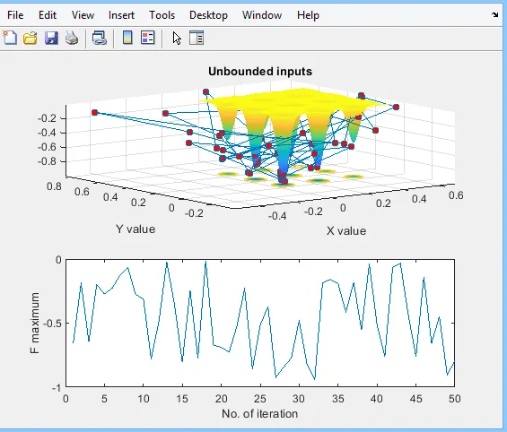
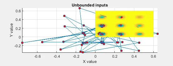
In this above figure, we see the various maxima points of each iteration in red dots but most of the points are out of the surface area of stalagmite function beacuse ga not consider itself the bounds of the search area.So, in the next study we specify the search area using lower nad upper bounds.

Case 2 is Statistical Behaviour with lower and upper bound

Observation: In this case same procedure is used but only change is in syntax of ga, we added lower and upper bound ([0;0],[1;1]) in the ga syntax to converge the area of ga.

RESULTS of 2nd case:

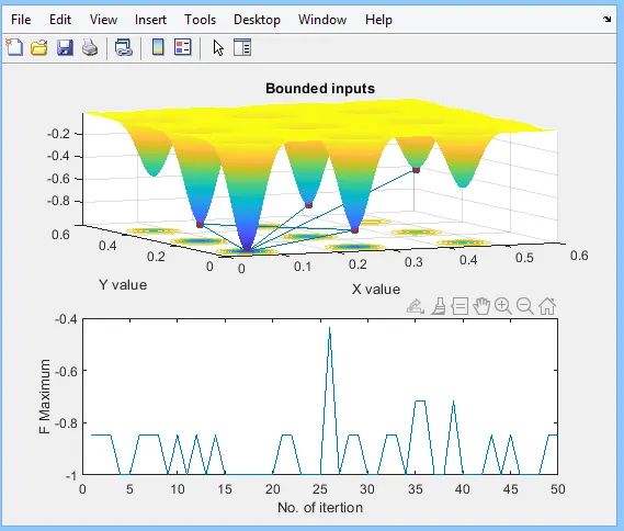
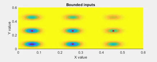
Observation: In this case we get better results from first case but the results is not yet converge to small area and in this case to optimise the data taken almost double time from previous case.

Case 3 case 2 with increase size of population from default value to 200.

For this case, use options in the ga syntax to change the default value of populationsize to 200.

syntax for change the default value of population size is

options = optimoptions(' SolverName,'Name','value').

RESULTS of 3rd case:

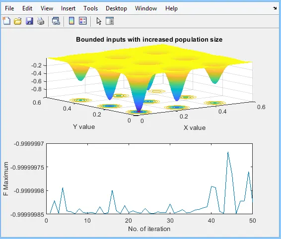
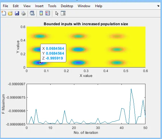
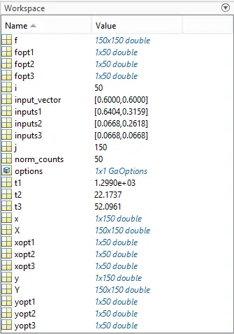
Observation: In this case we get the maxima of function at each iteration is concentrated to mainly one pionts but time taken to this optimization appro. 52 seconds which 5th times of the first case and 2.5 times of the second case.

Reference

https://in.mathworks.com/help/gads/what-is-the-genetic-algorithm.html

https://in.mathworks.com/help/gads/some-genetic-algorithm-terminology.html

https://in.mathworks.com/help/gads/genetic-algorithm-options.html#f8335

https://in.mathworks.com/help/gads/ga.html