Week 3 - Solving second order ODEs

Aim: To solve the ODE which represents the equation of motion of simple pendulum with damping.

Obejective: Write a program that solves the following ODE which represents the equation of motion of a simple pendulum with damping.

Theory: Simple Pendulum that moves in an oscillatory motion. It consists of a mass 'm' suspended by means of ligth inextensible string of length 'L' from a fixed support.The motion occurs in a vetical plane and is driven gravitational force.

Equation of motion;

In the above equation,

• g = gravity in m/s2,
• L = length of the pendulum in m,
• m = mass of the ball in kg,
• b=damping coefficient.

Since the equation is second order differential equation then first we will convert it into first oder differential equation to solve the ODE.

let,

`theta=theta1`

`d(theta1/dt)=theta2`

`d^2 theta/dt^2=d(theta2)/dt`

Code:

clear all
close all
clc

% Inputs 
b=0.05;       % damping coefficient
g=9.81;       % gravity in m/s^2
l=1;          % length of string in metre
m=1;          % mass of ball in kg

% initial condition
theta_0=[0;3];                 % angular displacement=0,angular velocity=3 rad/sec at time t=0.
t_span=linspace(0,20,200);   % break 20 seconds time span into 100 equal parts

% ode45 solver
[t,result]=ode45(@(t,theta) ode_funct(t,theta,b,g,l,m),t_span,theta_0);

%plotting
plot(t,result(:,1),'linewidth',3)
hold on
plot(t,result(:,2),'linewidth',3)
xlabel('time [seconds]')
legend('Angular Disp','Angular Velo.')


figure(2)
angularDisp=result(:,1);
ct=1;
for i=1:length(angularDisp)
    Adisp=angularDisp(i);
   %fixed end coordinate
    x0=0;
    y0=0;
    % free end coordinate
    x1=l*sin(Adisp);
    y1=-l*cos(Adisp);

    %plotting of string animation
    plot([-1.5 1.5],[0 0])
    hold on
    plot([x0 x1],[y0 y1],'linewidth',1,'color','c')
    %plotting of ball of mass 1 kg
    plot(x1,y1,'o','MarkerSize',10,'color','b')
    %fixed the axis
    axis([-1 1 -1.5 .5])
    xlabel('X Axis')
    ylabel('Y Axis')
    title('Animated pendulum')
    pause(0.0003)
    M(ct)=getframe(gcf);
    hold off
    ct=ct+1;
end
% create animation video of damped Simple Pendulum
movie(M)
Videofile=VideoWriter("pendul.avi","Uncompressed AVI");
open(Videofile)
writeVideo(Videofile,M)
close(Videofile)

Function code:

function [dtheta_dt]=ode_funct(t,theta,b,g,l,m)

theta1=theta(1);
theta2=theta(2);
dtheta1_dt=theta2;
dtheta2_dt=-(b/m)*theta2-(g/l)*sin(theta1);
dtheta_dt=[dtheta1_dt;dtheta2_dt];
end

Detail explanation of the program:

1. Write first three commands for clear workspace, close previous figure and clear command window.
2. Write inputs of the damped simple pendulum with intital condition and time span.
3. then write command to solve differential equation with the help of MATLAB inbuilt ODE solver function called ODE45 function.
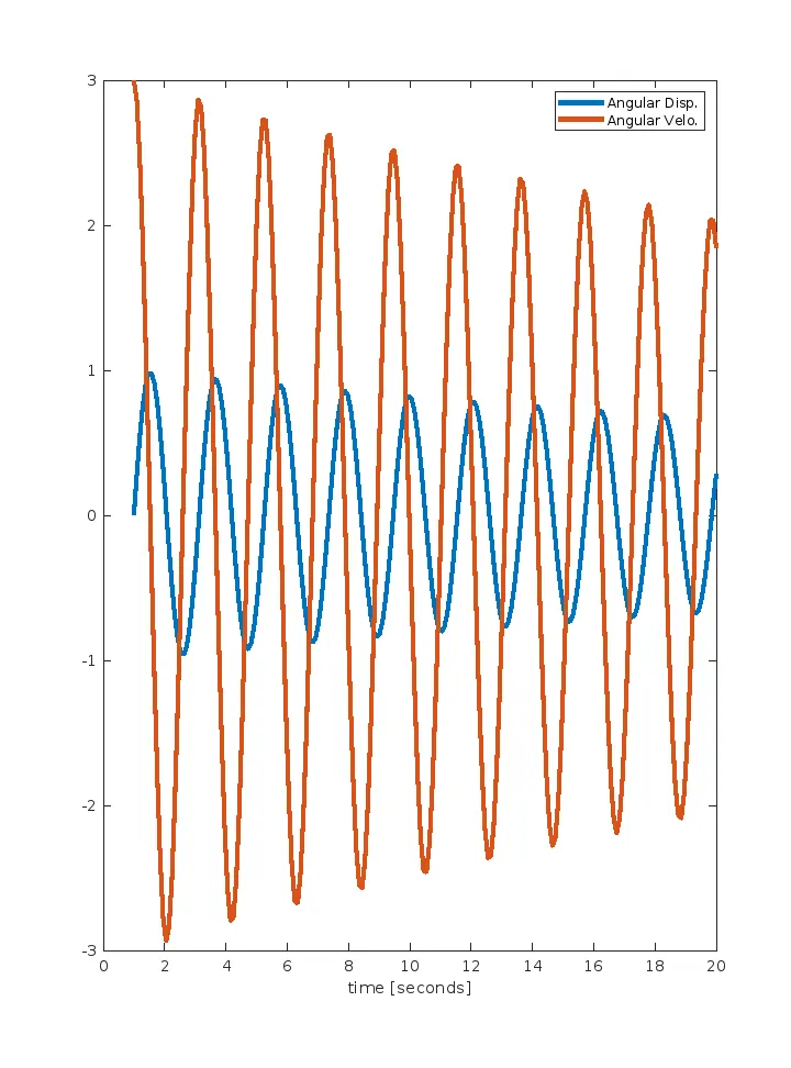
4. Write a command to plot the graph of both results i.e. Angular displacement and angular velocity of pendulum, with respects to time span.
5. Now write a for loop funnction to create the position of pendulum for each poisition of time.
6. then plot command is used to create the plot of simple pendulum (a string of 1 metre which one end fixed and other is free to air has a ball of mass 1kg)
7. then fix the axis of the plot by using axis command.
8. and last used create movie command to create animation of damped simple pendulum.

Movie command:

• Movie command is used to create animated video which collecting numbers of frames and make film.
• VideoWriter command is used specifies the name of the video file and type of data in which the moive stored.
• Open command is used to open the file.
• writeVideo command is used to create the video file.
• Close command is used too close the file.

ODE45 Solver:

ode45 is matlab inbuilt ODE solver used for medium order, non-stiff differential equations.

The syntax of ode45 solver is

[t,y] = ode45(odefun , tspan, y0)

It consists of output,ode function and input.

where,

[t,y] = Outputs

tspan and y0 = Inputs

tspan =[t(initial) t(final)]

y0= Initial condition

odefun = ode function

Results:

• A plot is drawn of angular displacement and angular velocity of the motion of simple pendulum in 0 to 20 seconds time frame.

plot

• The animation of simple pendulum which represent the which movement of the pendulum accorrding to the ordinary differential equation by using Matlab inbuilt ODE45 solver.

Animated video of simple pendulum

https://youtu.be/nQdEpkPzRVQ