Challenge

Week 4.1 - Genetic Algorithm

HHarthik T25 May 2022

Program to solve Genetic Algorithm

Abstract

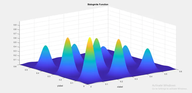
The main objective of this project is to optimise the stalagmite function and find the global maxima of the function and also the concept of genetic algorithm is also explained in this project by using matlab software.

The Following activities were done on this project,

Program 1 : Fitness Function
Program 2 : stalagmite function
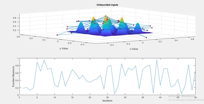
Program 3 : Unbounded Inputs
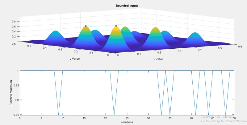
Program 4 : Bounded Inputs
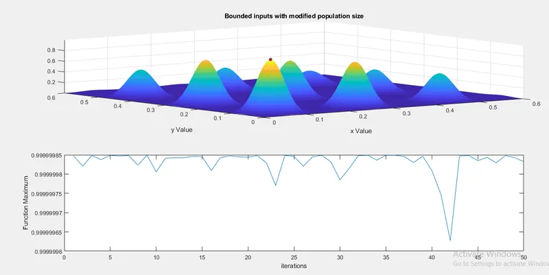
Program 5 : Bounded Inputs with modified population size
Program 6 : All in One program(combined),Except(program 1)

Keywords

Mat lab,Genetic algorithm,stalagmite function,Global maxima

Introduction

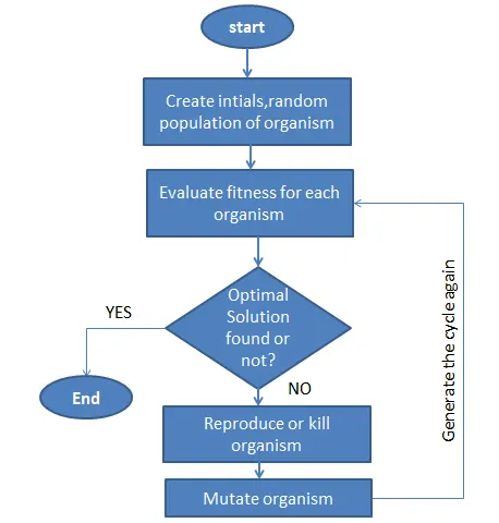
The concept of genetic algorithms is based on Darwin evolution therory,it is poineered by Holland.He was probably the first to use genetic operators such as the cross over,mutation,selection in the study of adaptive and artificial systems.Flow chart attached for reference,

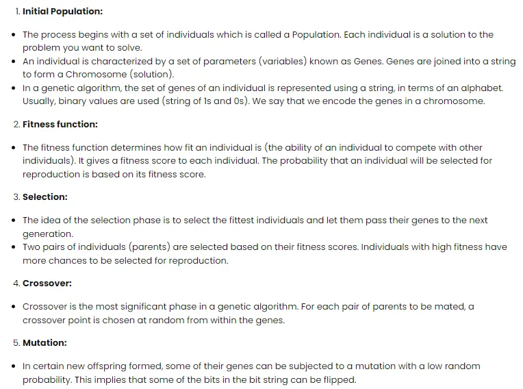
Genetic operators

1.Initial Population

2.Fitness Function

3.Selection operator

4.Crossover

5.Mutation

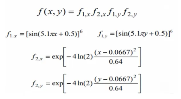
FORMULA:

FITNESS FUNCTION:

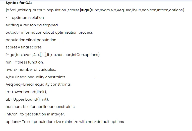
TERMS USED IN THIS PROJECT:

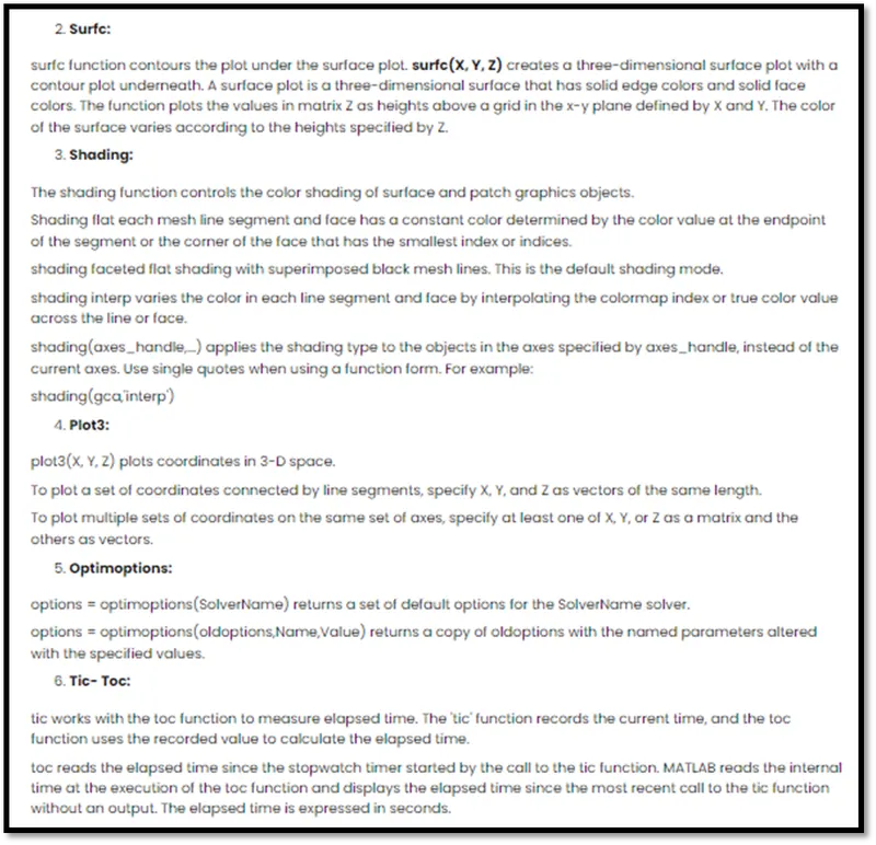
PROGRAM DONE USING MATLAB:

Program 1:

function [f]=stalagmite_function(input_vector)
x=input_vector(1);
y= input_vector(2);

% STEP-2(CALCULATION COMMANDS DEFINED IN PROGRAM)
f1=(sin(5.1*pi*x+0.5)).^6;
f2=(sin(5.1*pi*y+0.5)).^6;
f3=exp(-4.*log(2)*((x-0.0667).^2)./0.64);
f4=exp(-4.*log(2)*((y-0.0667).^2)./0.64);
f=-(f1*f2*f3*f4);
end

Program 2:

clear all
close all
clc

% STEP-1(INPUTS DEFINED IN PROGRAM)
% creating 1D arrays
x=linspace(0,0.6,150);
y=linspace(0,0.6,150);

% creating 2D arrays using one dimensional arrays
[x,y] = meshgrid(x,y);

% iteration count
num_cases=50;

% STEP-2(CALCULATION COMMANDS DEFINED IN PROGRAM)
% Evaluating the stalagmite function
for i=1:length(x)
    for j=1:length(y)
        input_vector(1)=x(i,j);
        input_vector(2)=y(i,j);
        f(i,j)=stalagmite_function(input_vector);
    end
end
% STEP-3(PLOTING COMMANDS FOR DIFFERENT GRAPH IN PROGRAM)
figure(1)
surfc(x,y,-f)

% to hide or remove the grid lines
shading interp
title('Stalagmite Function')
xlabel('xlabel')
ylabel('ylabel')
saveas(1,'Stalagmite Function.png')

Program 3:

% STEP-2(CALCULATION COMMANDS DEFINED IN PROGRAM)
% study 1:Unbounded/random sampling Inputs
tic
fopt(1:num_cases)= NaN;
xopt(1:num_cases)= NaN;
yopt(1:num_cases)= NaN;
for i=1:num_cases
    [inputs,fopt(i)]=ga(@stalagmite,2);
    xopt(i)=inputs(1);
    yopt(i)=inputs(2);
end

study1_time=toc;
% STEP-3(PLOTING COMMANDS FOR DIFFERENT GRAPH IN PROGRAM)
figure(2)
subplot(2,1,1)
surfc(x,y,-f)
hold on
shading interp
title('Unbounded inputs') 
plot3(xopt,yopt,-fopt,'marker','o','markersize',5,'markerfacecolor','r');
xlabel('x Value');
ylabel('y Value');

subplot(2,1,2)
plot(-fopt);
xlabel('iterations')
ylabel('Function Maximum')
saveas(2,'Unbound Inputs.png')

Program 4:

% STEP-2(CALCULATION COMMANDS DEFINED IN PROGRAM)
% study 2:Statistical Behaviour with upper and lower Bound Sampling
tic
fopt(1:num_cases)= NaN;
xopt(1:num_cases)= NaN;
yopt(1:num_cases)= NaN;
for i=1:num_cases
    [inputs,fopt(i)]=ga(@stalagmite,2,[],[],[],[],[0 0],[0.4 0.4]);
    xopt(i)=inputs(1);
    yopt(i)=inputs(2);
end

study2_time=toc;
% STEP-3(PLOTING COMMANDS FOR DIFFERENT GRAPH IN PROGRAM)
figure(3)
subplot(2,1,1)
surfc(x,y,-f)
hold on
shading interp
title('Bounded inputs') 
plot3(xopt,yopt,-fopt,'marker','o','markersize',5,'markerfacecolor','r');
xlabel('x Value');
ylabel('y Value');

subplot(2,1,2)
plot(-fopt);
xlabel('iterations')
ylabel('Function Maximum')
saveas(3,'Bounded Inputs.png')

Program 5:

% STEP-2(CALCULATION COMMANDS DEFINED IN PROGRAM)
% study 3:Code for upper and lower Bound Sampling and increase the
% population size
tic
options =optimoptions(@ga);
options=optimoptions(options,'populationsize',200);
fopt(1:num_cases)= NaN;
xopt(1:num_cases)= NaN;
yopt(1:num_cases)= NaN;
for i=1:num_cases
    [inputs,fopt(i)]=ga(@stalagmite,2,[],[],[],[],[0 0],[0.3 0.3],[],[],options);
    xopt(i)=inputs(1);
    yopt(i)=inputs(2);
end

study3_time=toc;
% STEP-3(PLOTING COMMANDS FOR DIFFERENT GRAPH IN PROGRAM)
figure(4)
subplot(2,1,1)
surfc(x,y,-f)
hold on
shading interp
title('Bounded inputs with modified population size') 
plot3(xopt,yopt,-fopt,'marker','o','markersize',5,'markerfacecolor','r');
xlabel('x Value');
ylabel('y Value');

subplot(2,1,2)
plot(-fopt);
xlabel('iterations')
ylabel('Function Maximum')
saveas(4,'Bounded Inputs.png')

global_maxima=-fopt

Program 6:

clear all
close all
clc

% STEP-1(INPUTS DEFINED IN PROGRAM)
% creating 1D arrays
x=linspace(0,0.6,150);
y=linspace(0,0.6,150);

% creating 2D arrays using one dimensional arrays
[x,y] = meshgrid(x,y);

% iteration count
num_cases=50;

% STEP-2(CALCULATION COMMANDS DEFINED IN PROGRAM)
% Evaluating the stalagmite function
for i=1:length(x)
    for j=1:length(y)
        input_vector(1)=x(i,j);
        input_vector(2)=y(i,j);
        f(i,j)=stalagmite_function(input_vector);
    end
end
% STEP-3(PLOTING COMMANDS FOR DIFFERENT GRAPH IN PROGRAM)
figure(1)
surfc(x,y,-f)

% to hide or remove the grid lines
shading interp
title('Stalagmite Function')
xlabel('xlabel')
ylabel('ylabel')
saveas(1,'Stalagmite Function.png')

% STEP-2(CALCULATION COMMANDS DEFINED IN PROGRAM)
% study 1:Unbounded/random sampling Inputs
tic
fopt(1:num_cases)= NaN;
xopt(1:num_cases)= NaN;
yopt(1:num_cases)= NaN;
for i=1:num_cases
    [inputs,fopt(i)]=ga(@stalagmite,2);
    xopt(i)=inputs(1);
    yopt(i)=inputs(2);
end

study1_time=toc;
% STEP-3(PLOTING COMMANDS FOR DIFFERENT GRAPH IN PROGRAM)
figure(2)
subplot(2,1,1)
surfc(x,y,-f)
hold on
shading interp
title('Unbounded inputs') 
plot3(xopt,yopt,-fopt,'marker','o','markersize',5,'markerfacecolor','r');
xlabel('x Value');
ylabel('y Value');

subplot(2,1,2)
plot(-fopt);
xlabel('iterations')
ylabel('Function Maximum')
saveas(2,'Unbound Inputs.png')

% STEP-2(CALCULATION COMMANDS DEFINED IN PROGRAM)
% study 2:Statistical Behaviour with upper and lower Bound Sampling
tic
fopt(1:num_cases)= NaN;
xopt(1:num_cases)= NaN;
yopt(1:num_cases)= NaN;
for i=1:num_cases
    [inputs,fopt(i)]=ga(@stalagmite,2,[],[],[],[],[0 0],[0.4 0.4]);
    xopt(i)=inputs(1);
    yopt(i)=inputs(2);
end

study2_time=toc;
% STEP-3(PLOTING COMMANDS FOR DIFFERENT GRAPH IN PROGRAM)
figure(3)
subplot(2,1,1)
surfc(x,y,-f)
hold on
shading interp
title('Bounded inputs') 
plot3(xopt,yopt,-fopt,'marker','o','markersize',5,'markerfacecolor','r');
xlabel('x Value');
ylabel('y Value');

subplot(2,1,2)
plot(-fopt);
xlabel('iterations')
ylabel('Function Maximum')
saveas(3,'Bounded Inputs.png')

% STEP-2(CALCULATION COMMANDS DEFINED IN PROGRAM)
% study 3:Code for upper and lower Bound Sampling and increase the
% population size
tic
options =optimoptions(@ga);
options=optimoptions(options,'populationsize',200);
fopt(1:num_cases)= NaN;
xopt(1:num_cases)= NaN;
yopt(1:num_cases)= NaN;
for i=1:num_cases
    [inputs,fopt(i)]=ga(@stalagmite,2,[],[],[],[],[0 0],[0.3 0.3],[],[],options);
    xopt(i)=inputs(1);
    yopt(i)=inputs(2);
end

study3_time=toc;
% STEP-3(PLOTING COMMANDS FOR DIFFERENT GRAPH IN PROGRAM)
figure(4)
subplot(2,1,1)
surfc(x,y,-f)
hold on
shading interp
title('Bounded inputs with modified population size') 
plot3(xopt,yopt,-fopt,'marker','o','markersize',5,'markerfacecolor','r');
xlabel('x Value');
ylabel('y Value');

subplot(2,1,2)
plot(-fopt);
xlabel('iterations')
ylabel('Function Maximum')
saveas(4,'Bounded Inputs.png')

global_maxima=-fopt

EXPLANATION OF CODE

STEP-1(INPUTS DEFINED IN PROGRAM)

Program 2:
X & y values determined.
Iteration count determined

STEP-2(CALCULATION COMMANDS DEFINED IN PROGRAM)

Program 1:
Fitness Function formula defined.
Program 2:
Function calling defined.
Program 3:
Unbounded /random sampling Inputs calculated.
Program 4:
Statistical Behaviour with upper and lower Bound Sampling calculated.
Program 5:
Code for upper and lower Bound Sampling and increase the population size.

STEP-3(PLOTING COMMANDS FOR DIFFERENT GRAPH IN PROGRAM)

Program 2:
stalagmite plotted.
Program 3:
Unbounded /random sampling Inputs plotted.
Program 4:
Statistical Behaviour with upper and lower Bound Sampling plotted.
Program 5:
Code for upper and lower Bound Sampling and increase the population size plotted.

ERRORS FACED WHILE PROGRAMMING:

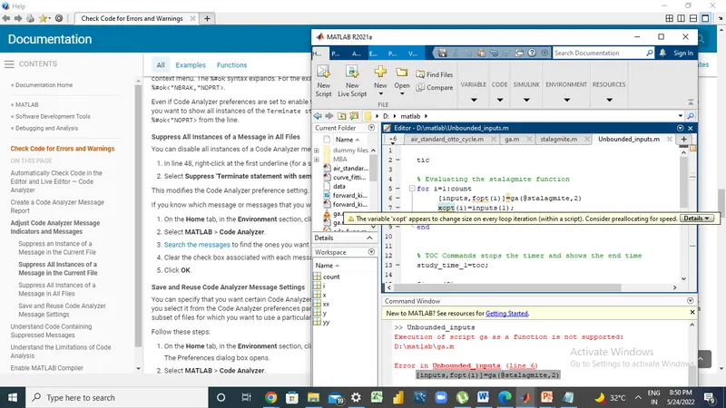
To solve this issue the following commands were used.
fopt(1:num_cases)= NaN;
xopt(1:num_cases)= NaN;
yopt(1:num_cases)= NaN;

CONCLUSIONS WITH RESULTS:

Output for program(2,3,4,5):

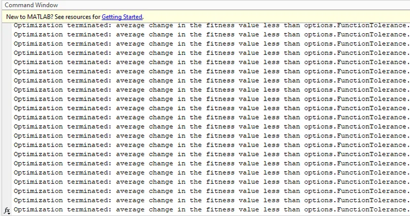
Output for program 5:

Global Maxima values shown below.

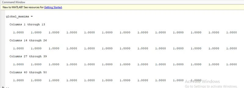
RESULTS:

Program 2 (Graph):

Program 3 (Graph):

Program 4 (Graph):

Program 5 (Graph):

REFERENCES:

https://en.wikipedia.org/wiki/Stalagmite

https://in.mathworks.com/help/matlab/matlab_env/add-remove-or-reorder-folders-on-the-search-path.html

https://stackoverflow.com/questions/28408332/attempt-to-execute-script-as-a-function

https://towardsdatascience.com/introduction-to-genetic-algorithms-including-example-code-e396e98d8bf3

Week 4.1 - Genetic Algorithm

Ship work like this
in your own course.

Talk to a career counsellor

Ship work like thisin your own course.

Talk to a career counsellor

Ship work like this
in your own course.