Week 3 - Solving second order ODEs
Program to solve 2nd order ODEs
Abstract
The main objective of this project is to solve the given equation and to plot the results. In this project the 2nd order ODEs is considered, which represents the equation of motion of simple pendulum with damping. And the program was divided into two parts ,where the main program consist of calculations and plotting commands and another one has ODEs calculations using function. These 2 programs were done by Matlab software.
Keywords
Mat lab,ODEs,1st order ODE,2nd order ODE,Simple pendulum
Introduction
In this program, 2nd order ODEs (motion of simple pendulum with damping) were considered
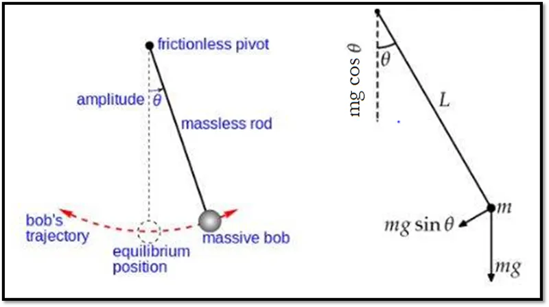
ODEs are a differential equation containing one or more functions of one independent variable and the derivatives of those functions. In this project the simple pendulum ODE is considered. In the simple pendulum there is a weight (or bob) n the end of a massless cord suspended from a pivot without friction. When initial push is applied it swings.
Input Data
Damping coefficient (b) - 0.05 (value taken from question)
Length of movable rod (L) - 1.2 m (assumed)
Mass of bob (m) - 1 Kg (value taken from question)
gravity (g) - 9.81 m/s^2
time span (t_span) - 0 to 20 (value taken from question),with 250 interval (assumed)
displacement - 0 (value taken from question)
velocity - 3 rad/sec (value taken from question)
FORMULA
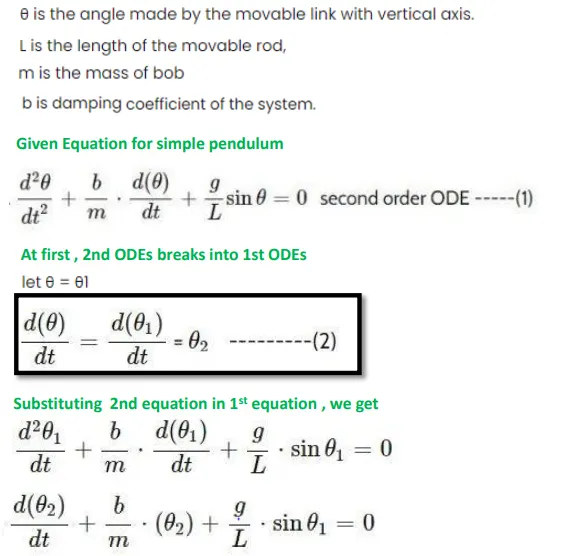
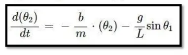
In Function program,the 2nd order ODE to 1st order ODE.
This Equation is calculated and solved by using Function.
In Main program,ode45 in built function used to solve this project and the function program is also called here.

PROGRAM USING MATLAB
1st Program (Function)-2nd order ODEs splited into two 1st order ODEs
function[dtheta_dt]=ode_fun(t,theta,b,g,l,m)
% STEP-2(CALCULATION COMMANDS DEFINED IN PROGRAM)
% ODE problem definition were done in below steps
% theta(1) is defined as the angular displacement and it is assigned to theta1
% theta(2) is defined as the angular velocity and it is assigned to theta2

    theta1 = theta(1);
    theta2 = theta(2);

%     in this the 2nd order ODE is splited into two 1st order ODEs
    dtheta1_dt = theta2;
    dtheta2_dt = -(b/m)*theta2 - (g/l)*sin(theta1);
    dtheta_dt=[dtheta1_dt;dtheta2_dt];
end
2nd Program (Main) - Calling the Function with plots and simulation
clear all
close all
clc

% STEP 1:INPUTS DEFINED IN PROGRAM
% inputs for (Length of movable rod(L) were assumed)
% inputs for taken from question
% Damping coefficient (b),Mass of bob (m),time span (t_span),displacement,velocity)

b=0.05;
g=9.81;
l=1.2;
m=1;
% displacement and velocity values (0 and 3) were taken from question
theta_0=[0;3];
% time span 0 to 20
t_span=linspace(0,20,250);

% STEP-2(CALCULATION COMMANDS DEFINED IN PROGRAM)
% ODE problem calling the function were done in below step
[t,results]=ode45(@(t,theta)ode_func(t,theta,b,g,l,m),t_span,theta_0)

% STEP-3(PLOTING COMMANDS FOR DIFFERENT GRAPH IN PROGRAM)
% Two output were displayed
% one is plotting angular velocity/ displacement to time in sec
% plotting 1st output
figure(1);
plot(t,results(:,1));
hold on;
plot(t,results(:,2));
title('Hormonic Motion of Pendulum');
xlabel('time in sec');
ylabel('angular velocity (rad/s)/displacement(rad)');
legend('displacement','angular velocity');


% another one is simulating the simple pendulum motion using movie command
ct=1;

for i=1 :length(t);
%     inital position of pendulum defined
    x0=0;
    y0=0;

%     Final position of pendulum defined
    x1=1*sin(results(i,1));
    y1=-1*cos(results(i,1));

%     plotting 2nd output
    figure(2);

%     to plot pendulum string
    plot([x0 x1],[y0 y1],'markersize',8,'linewidth',3,'color','r');
    hold on;

%     to plot center point of fixed line
    plot([0 0],[0 0],'o','markerfacecolor','k','markersize',8);

%     to plot the fixed line
    plot([-2 2],[0,0],'linewidth',4,'color','b');

%     to plot the ball at end of penduum string
    plot(x1,y1,'r-o','MarkerSize',22,'markerfacecolor','g');
    axis([-2 2 -2 2]);
    title('Simulation of Simple Pendulum');
    legend('Length of movable rod(L)','center point of fixed line','Fixed End','BOB(Movable end)');
    hold off;

%     to simulate the program movie command is used
    M(ct)=getframe(gcf);
    ct=ct+1;

end

movie(M);
Videofile=VideoWriter('simple_pendulum.avi','uncompressed AVI');
open(Videofile);
writeVideo(Videofile,M);
close(Videofile);
EXPLANATION OF CODE
STEP-1(INPUTS DEFINED IN PROGRAM)
- b,g,l,m,displacent,velocity,time span defined.
- In time span linspace command is used.
- semicolon is used , not to display the values in output
STEP-2(CALCULATION COMMANDS DEFINED IN PROGRAM)
- Calculation are done by using two seperate program
- Function and main program
- In Function program, 2nd order ODE is splited into two 1st order ODEs. here, ODE problem definition were done
- dtheta1_dt = theta2;
dtheta2_dt = -(b/m)*theta2 - (g/l)*sin(theta1); - In Main program,Calling the function were done.
- [t,results]=ode45(@(t,theta)ode_func(t,theta,b,g,l,m),t_span,theta_0)
- semicolon is not used in this line, to display the values in output box
STEP-3(PLOTING COMMANDS FOR DIFFERENT GRAPH IN PROGRAM)
- Two otput were displayed.
- one is plotting angular velocity/ displacement to time in sec
- axis,xlabel, ylabel,title commands are used for better understanding of graph.
- another one is simulating the simple pendulum motion using movie command
- to save the simulation as a video file some commands are used. which are defined in program.
ERRORS FACED WHILE PROGRAMMING
- No Errors were found while programming
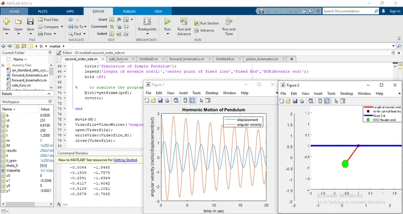
- Screenshot attached for reference.
OUTPUT
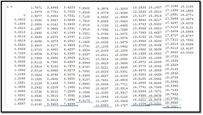
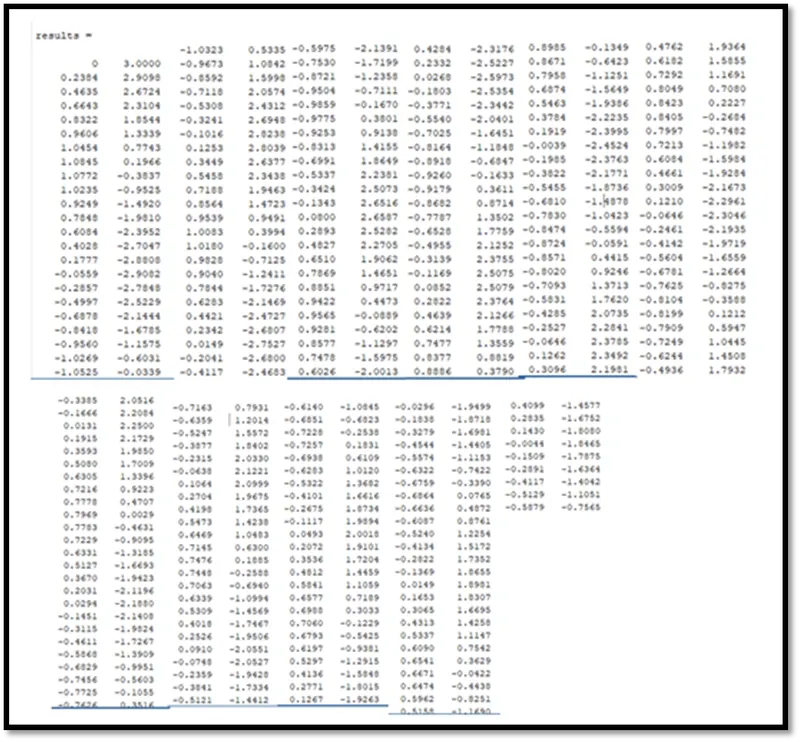
- t and results values are shown below.
- Screenshot attached for reference.
RESULTS
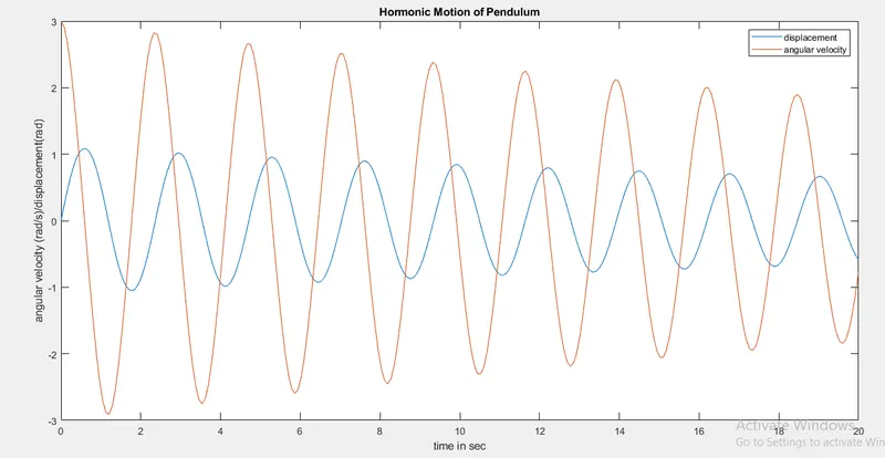
- plotting angular velocity/ displacement to time in sec.
- Screenshot attached for reference.
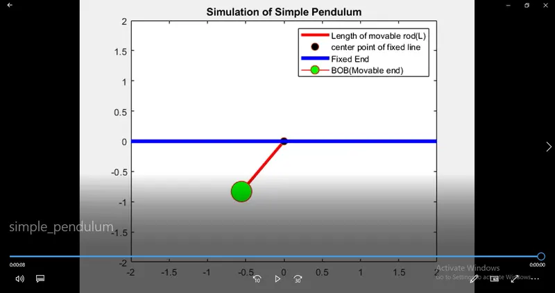
- Simulating the program using movie command.
- Screenshot attached for reference.
Conclusion
- plotting angular velocity/ displacement to time in sec.
- Simulating the program using movie command.
- Link attached for reference.
YouTube link
Google drive link
https://drive.google.com/file/d/1G-DzVIplWf1k-Vft1OXxV_0wcEo4SFNb/view?usp=sharing