Week 4.1 - Genetic Algorithm
GENETIC ALGORITHM
AIM:
- To write a code in MATLAB to optimise the stalagmite function and find the global maxima of the function.
- To explain the syntax for ga in MATLAB.
- To plot graphs for all 3 studies and for F maximum vs no. of iterations.
THEORY:
STALAGMITE
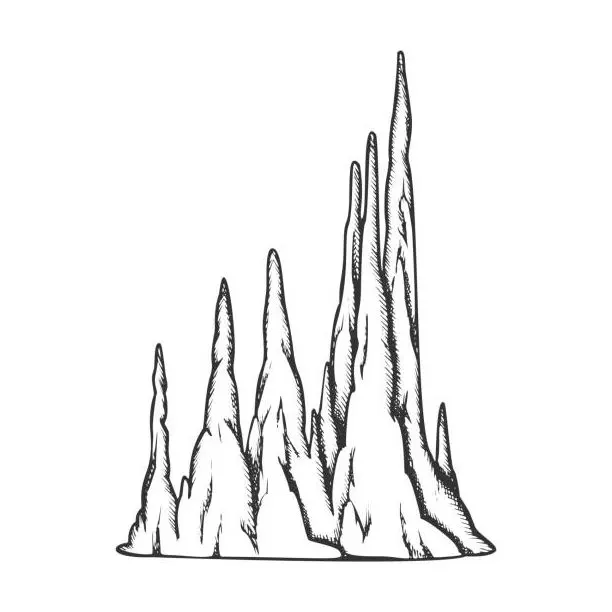
- A stalagmite is an upward-growing mound of mineral deposits that have precipitated from water dripping onto the floor of a cave. Most stalagmites have rounded or flattened tips.
- There are some mathematical functions which represents shapes similar to stalagmites.
- A stalagmite function generally refers to the function with which we are generating values over a stalagmite kind of surface for finding out the local and global maxima and minima of that particular function.
GENETIC ALGORITHM (GA)
Nature has always been a great source of inspiration to all mankind. Genetic Algorithm is a search based optimization technique, based on the principle of Genetics and Natural Selection. GA's are a subset of a much larger branch of computation known as Evolutionary Computation. It's frequently used to find optimal or near optimal solutions to difficult problems which otherwise would take a lifetime to solve. GA's were developed by John Holland and his students and collegues at the university of Michigan.
In GA's, we have a pool or a population of possible solutions to the given problem. These solutions then undergo recombination and mutation, producing new children, and the process is repeated over various generation.
Basic structure of Genetic Algorithm
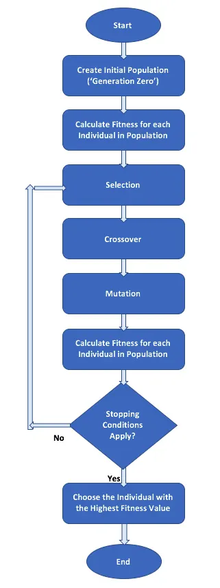
- Initial Population - There will be a initial population of possible solutions to the given prolem.
- Fitness Calculation - Each individual solution is taken as input to perform a fitness function and the output will be a fitness value which gives an idea on how much 'fit' the indiidual solutions are.
- Selection - The best fit is considered to be parent and the generating some childrens or can say offsprings. These include Cross over, Mutation etc.
- Cross over - It Produces offspring by swapping parts or genes of the chromosomes. Crossover has a higher probability, typically 0.8-0.95.
- Mutation - It produces offsprings by flipping some digits of a string, which generates new solutions. Then fitness calculations are again done to select best offspring.
If the selected offspring gives a best output the problem is solved otherwise, the loop will continue again by transferring newly generated offsprings to the population by replacing the current population.
EQUATIONS USED
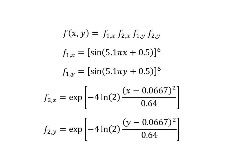
This equation is used in the stalagmite function to plot the graph while running the main program
CODE TO OPTIMISE THE STALAGMITE FUNCTION AND TO FIND GLOBAL MAXIMA OF THE FUNCTION
STALAGMITE FUNCTION
function [f] = get_stalagmite(input_vector) %function created naming 'get_stalagmite' by providing 'input_vector' as input

%finding f1x
term1 = 5.1*pi.*input_vector(1)+0.5;
a = (sin(term1)).^6

%finding f1y
term2 = 5.1*pi.*input_vector(2)+0.5;
b = (sin(term2)).^6

%finding f2x
term3 = ((input_vector(1) - 0.0667).^2)/0.64;
c = exp(-4*log(2).*term3)

%finding f2y
term4 = ((input_vector(2)-0.0667).^2)/0.64;
d = exp(-4*log(2).*term4)

f = a*b*c*d %output of the function is assigned to [f]

end
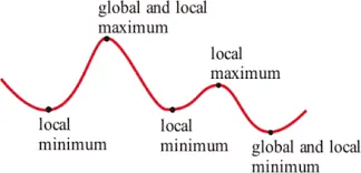
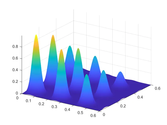
Shows a function created to solve the equations to find the different values of "z" coordinate with respective to the "x" and "y" coordinates. Simply can say this determine the height of the stalagmite at each points of x and y coordinate. The point at which "z" coordinate is greater is global maxima and where it's smaller is global minima while considering globally. There are also local maxima and local minima where "z" coordinate is maximum and "z" coordinate is minimum respectively when we consider locally. An inbuilt function Genetic Algorithm (ga) will help to find the global minima and by altering the certain equation we can find the peak value which is global maxima. In the below figure will gives an idea on those points.
CODE TO FIND GLOBAL MINIMA
clear all
close all
clc

%defining our search space
x = linspace(0,0.6,150);
y = linspace(0,0.6,150);

%creating a 2dimensional array
[xx yy] = meshgrid(x,y);

%for loop
for i = 1 : length(xx);                       %variable 'i' is assigned with different values from 1 to length of XX
    for j = 1 : length(yy);                   %variable 'j' is assigned with different values from 1 to length of YY
        input_vector(1) = xx(i,j);            %the value of XX from each iteration is assigned to input_vector(1)
        input_vector(2) = yy(i,j);            %the value of YY from each iteration is assigned to input_vector(2)
        f (i,j) = get_stalagmite(input_vector);   %the input_vector 1 and 2 are given as input while calling the function to solve the required formula

    end  %for loop ends
end      %for loop ends

 surfc(xx,yy,f)                     %to visualize how the data looks in 3D
 shading interp                     %which will remove the grid lines in the surface plot

 [input, fval] = ga(@get_stalagmite,2)  %GA helps to find the minimum values for get_stalagmite function
OUTPUT :
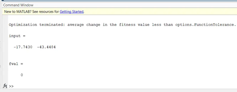
In the command window we can find fval = 0 which represents the global minima and input = -17.7430 , -43.4484 are the "x" and "y" coordinate respectievely.
CODE TO FIND GLOBAL MAXIMA
1) STATISTICAL BEHAVIOUR
clear all
close all
clc

%defining our search space
x = linspace(0,0.6,150);  %search space for x value is input by linspace from 0 to 0.6 having in a 150 evenly spaced sequence
y = linspace(0,0.6,150);  %search space for y value is input by linspace from 0 to 0.6 having in a 150 evenly spaced sequence

[XX YY] = meshgrid(x,y);  %to create a 2D array

for i = 1 : length(XX)                          %variable 'i' is assigned with different values from 1 to length of XX
    for j = 1 : length(YY)                      %variable 'j' is assigned with different values from 1 to length of YY
        input_vector(1) = XX(i,j);              %the value of XX from each iteration is assigned to input_vector(1)
        input_vector(2) = YY(i,j);              %the value of YY from each iteration is assigned to input_vector(2)
        f (i,j)= get_stalagmite(input_vector);  %the input_vector 1 and 2 are given as input while calling the function to solve the required formula

    end  %for loop ends
end      %for loop ends


num_cases = 50;  %a variable num_cases is introduced and assigned a value of 50 as it's used to control the number of iterations in this code


%study 1 - statistical behaviour
tic
for i = 1 : num_cases;                           %variable 'i' is assigned with different values from 1 to num_cases
    [inputs, fopt(i)] = ga(@get_stalagmite, 2)   %GA helps to find the minimum values for get_stalagmite function.
    xopt(i) = inputs(1);                         %the input(1) is stored to xopt(i)
    yopt(i) = inputs(2);                         %the input(2) is stored to yopt(i)
end                                              %for loop ends
studytime1 = toc

figure(1)                                        %figure 1 introduced
subplot(2,1,1)                                   %to create subplots in a given figure
surfc(XX,YY,f)                                   %to visualize how the data looks in 3D
shading interp                                   %which will remove the grid lines in the surface plot
xlabel('x axis')                                 %naming x axis
ylabel('y axis')                                 %naming y axis
zlabel('z axis')                                %naming z axis
title('3D REPRESENTATION OF THE FUNCTION')       %naming title of the diagram
hold on                                          %holds the initial plot created
plot3(xopt,yopt,fopt,'marker','o','markersize',5,'markerfacecolor','r')  %to create a 3D plot
subplot(2,1,2)                                                           %to form another subplot in the same figure window
plot(fopt)                                                               %to plot the variation of fopt
title('ITERATION VS FUNCTION MINIMA')                                    %naming the title
xlabel('iterations')                                                     %naming x-axis
ylabel('function minimum')                                               %naming y-axis
OUTPUT :
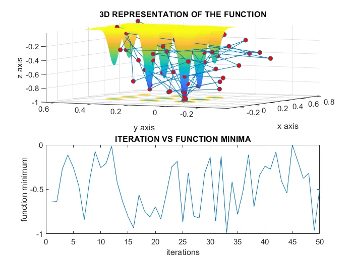
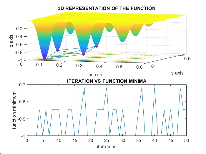
- Optimal values obtained varies from 0 to -1 for 50 iterations.
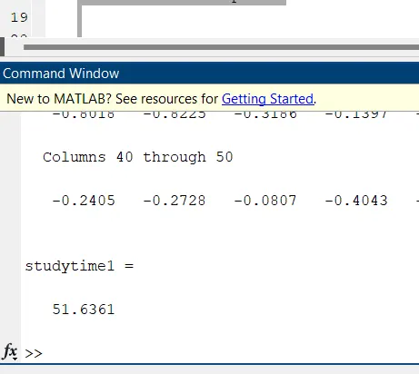
- Study time took about 51.6361 seconds
Code is performed for 50 iterations of ga and from each iteration different values of optimum value for 'f' which is global maxima has been got, which is wrong. From the function minima vs iterations graph there can see the value is changing for each iteration. As the ga don't know the lower and upper bound that's why ga found values other than from the out of the graph as shown below. In the next code there will assign the required upper and lower bounds then ga can find global maxima more efficiently.
2) STATISTICAL BEHAVIOUR WITH UPPER AND LOWER BOUND
clear all
close all
clc

%defining our search space
x = linspace(0,0.6,150);  %search space for x value is input by linspace from 0 to 0.6 having in a 150 evenly spaced sequence
y = linspace(0,0.6,150);  %search space for y value is input by linspace from 0 to 0.6 having in a 150 evenly spaced sequence

[XX YY] = meshgrid(x,y);  %to create a 2D array

for i = 1 : length(XX)                          %variable 'i' is assigned with different values from 1 to length of XX
    for j = 1 : length(YY)                      %variable 'j' is assigned with different values from 1 to length of YY
        input_vector(1) = XX(i,j);              %the value of XX from each iteration is assigned to input_vector(1)
        input_vector(2) = YY(i,j);              %the value of YY from each iteration is assigned to input_vector(2)
        f (i,j)= get_stalagmite(input_vector);  %the input_vector 1 and 2 are given as input while calling the function to solve the required formula

    end  %for loop ends
end      %for loop ends


num_cases = 50;  %a variable num_cases is introduced and assigned a value of 50 as it's used to control the number of iterations in this code

%study -2 statistical behaviour - with upper and lower bounds
tic
for i = 1 : num_cases                                                     %variable 'i' is assigned with different values from 1 to num_cases
    [inputs fopt(i)] = ga(@get_stalagmite,2,[],[],[],[],[0;0],[1;1]);     %GA helps to find the minimum values for get_stalagmite function
    xopt(i) = inputs(1);                                                  %the input(1) is stored to xopt(i)
    yopt(i) = inputs(2);                                                  %the input(2) is stored to yopt(i)
end                                                                       %for loop ends
studytime2 = toc

figure(2)                                        %figure 1 introduced
subplot(2,1,1)                                   %to create subplots in a given figure
surfc(XX,YY,f)                                   %to visualize how the data looks in 3D
xlabel('x axis')                                 %naming x axis
ylabel('y axis')                                 %naming y axis
zlabel('z axis')                                %naming z axis
title('3D REPRESENTATION OF THE FUNCTION')       %naming title of the diagram
shading interp                                   %which will remove the grid lines in the surface plot
hold on                                          %holds the initial plot created
plot3(xopt,yopt,fopt,'marker','o','markersize',5,'markerfacecolor','r')  %to create a 3D plot
subplot(2,1,2)                                                           %to form another subplot in the same figure window
plot(fopt)                                                               %to plot the variation of fopt
title('ITERATION VS FUNCTION MINIMA')                                    %naming the title
xlabel('iterations')                                                     %naming x-axis
ylabel('function minimum')                                               %naming y-axis
OUTPUT :
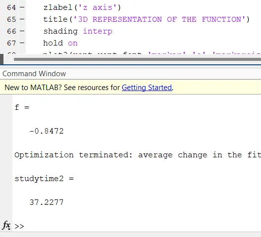
- Optimal values obtained varies from 0.7 to -1 for 50 iterations.
- Study time took about 37.2277 seconds
Comparing with the above case the value for the global maxima almost approaches to it's peak value and hence found values between 0.7 and -1. In the next code there will increase the number of population size so it will give more accurate result.
3) INCREASING GA ITERATIONS
clear all
close all
clc

%defining our search space
x = linspace(0,0.6,150);  %search space for x value is input by linspace from 0 to 0.6 having in a 150 evenly spaced sequence
y = linspace(0,0.6,150);  %search space for y value is input by linspace from 0 to 0.6 having in a 150 evenly spaced sequence

[XX YY] = meshgrid(x,y);  %to create a 2D array

for i = 1 : length(XX)                          %variable 'i' is assigned with different values from 1 to length of XX
    for j = 1 : length(YY)                      %variable 'j' is assigned with different values from 1 to length of YY
        input_vector(1) = XX(i,j);              %the value of XX from each iteration is assigned to input_vector(1)
        input_vector(2) = YY(i,j);              %the value of YY from each iteration is assigned to input_vector(2)
        f (i,j)= get_stalagmite(input_vector);  %the input_vector 1 and 2 are given as input while calling the function to solve the required formula

    end  %for loop ends
end      %for loop ends


num_cases = 50;  %a variable num_cases is introduced and assigned a value of 50 as it's used to control the number of iterations in this code

%study 3 increasing GA iterations
options = optimoptions('ga')
options = optimoptions(options,'PopulationSize',170)

tic
for i = 1 : num_cases                                                                 %variable 'i' is assigned with different values from 1 to num_cases
    [inputs fopt(i)] = ga(@get_stalagmite,2,[],[],[],[],[0;0],[1;1],[],[],options);   %GA helps to find the minimum values for get_stalagmite function
    xopt(i) = inputs(1);                                                              %the input(1) is stored to xopt(i)
    yopt(i) = inputs(2);                                                              %the input(2) is stored to yopt(i)
end                                                                                   %for loop ends
studytime3 = toc

figure(3)                                        %figure 1 introduced
subplot(2,1,1)                                   %to create subplots in a given figure
surfc(XX,YY,f)                                   %to visualize how the data looks in 3D
xlabel('x axis')                                 %naming x axis
ylabel('y axis')                                 %naming y axis
zlabel('z axis')                                %naming z axis
title('3D REPRESENTATION OF THE FUNCTION')       %naming title of the diagram
shading interp                                   %which will remove the grid lines in the surface plot
hold on                                          %holds the initial plot created
plot3(xopt,yopt,fopt,'marker','o','markersize',5,'markerfacecolor','r')  %to create a 3D plot
subplot(2,1,2)                                                           %to form another subplot in the same figure window
plot(fopt)                                                               %to plot the variation of fopt
title('ITERATION VS FUNCTION MINIMA')                                    %naming the title
xlabel('iterations')                                                     %naming x-axis
ylabel('function minimum')                                               %naming y-axis
OUTPUT :
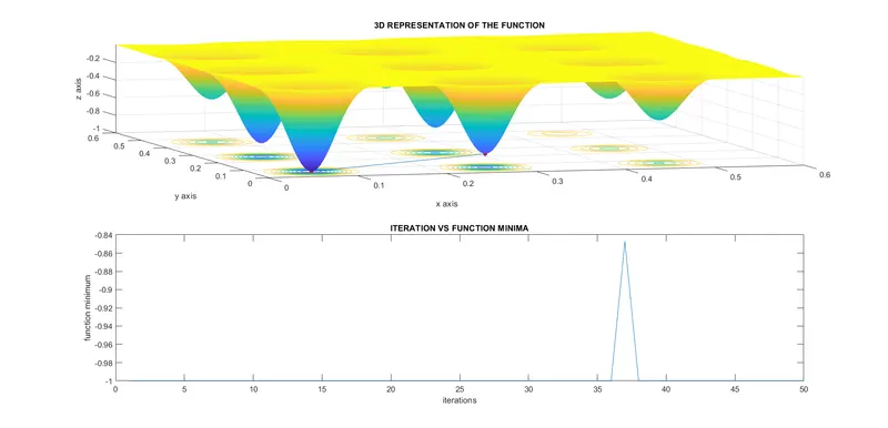
- Optimal values obtained varies from 0.7 to -1 for 50 iterations but almost in all iterations except iterations between 37 to 39 got a peak value of -1.
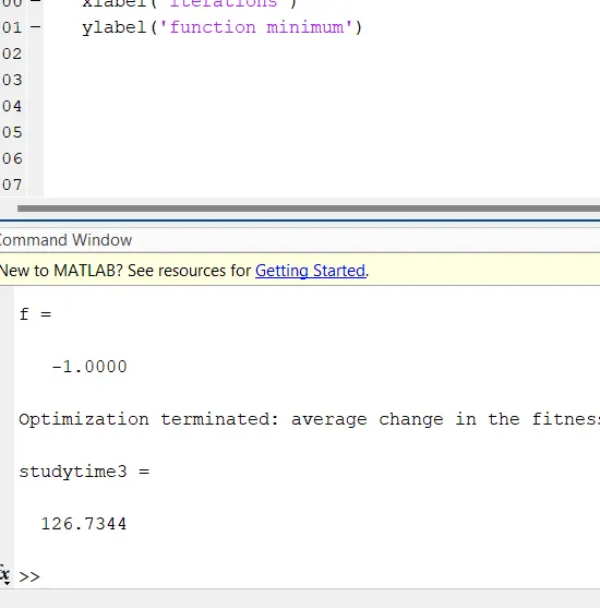
- Study time took about 126.7344 seconds.
In GA, the population size is an important parameter which directly influences the ability to search an optimum solution in the search space. Having a large number of population leads to the accuracy of getting an optimal solution.
GENETIC ALGORITHM SYNTAX :
x = ga (fun, nvars, A, b, Aeq, beq, lb, ub, nonIcon, options)
- x : It represents the local minima.
- ga : It is an inbuilt function called "Genetic Algorithm". It is used to find the minimum of a function.
- fun : It is the objective function to be solved. (here it's "get_stalagmite")
- nvars : It is the dimension of the function. (here it's 2)
- A and b : They are used to represent any linear inequalities that present in the function. (here there is no linear inequalities, so A =[] and b = [])
- Aeq and beq : They are used to represent any linear equalities that present in the function. (here there is no linear equalities, so Aeq =[] and beq = [])
- lb : Lower bound. (here it's 0)
- up : Upper bound. (here it's 1)
- nonIcon : Represents non linear constraints (here there is no nonlinear constarints, therefore nonIcon =[])
- options : It's used for additional operations like population size, population type, crossover fcn ...etc (here introduced population size about 170)
STOPING CRITERIA :
The number of iterations in an optimization depends on a solver's stopping criteria. These criteria include several tolerances you can set. Generally, a tolerance is a threshold which, if crossed, stops the iterations of a solver. Here in each set a stopping criteria of 50 iterations has been given input, so after 50 iterations the ga stops and produce output.
There are different stopping criterias for example Maxgenerations, Maxtime, Fitnesslimit.. etc.
-
Maxgenerations — The algorithm stops when the number of generations reaches MaxGenerations.
-
MaxTime — The algorithm stops after running for an amount of time in seconds equal to MaxTime.
-
FitnessLimit — The algorithm stops when the value of the fitness function for the best point in the current population is less than or equal to FitnessLimit
EXPLANATION :
- Firstly, the required function code has been created as shown. It's to be noted that the function name and the file name should be same.
- In a new tab, starting with the usual commands clear all, close all and clc, the necessary search space has been created and then converted into 2D array by meshgrid command.
- For loops has been introduced to find the i,j entry of each 2D array and found the corresponding values at each i,j entries and given as input to the get_stalagmite function.
STATISTICAL BEHAVIOUR
- Considering 50 numbers of iterations, then a for loop is introduced with variable 'i' having values from 1 to length of iteration.
- Then an inbuilt function, "genetic algorithm" (ga) is called to solve the "get_stalagmite function.
- Corresponding optimum values of "x" , "y" and f is found from each iteration. The tic and toc command is used to find the time required to run the code. The necessary plotting is done.
STATISTICAL BEHAVIOUR WITH UPPER AND LOWER BOUND
- In this case ga syntax has been modified by introducing lower and upper bounds.
GA ITERATION IS INCREASED
- In this case the ga syntax has been modified by introducing population size.