Project 2 - Rankine cycle Simulator

RANKINE CYCLE SIMULATOR

AIM :

• To create a Rankine Cycle Simulator using MATLAB.
• To calculate the state points of the Rankine Cycle based on user inputs.
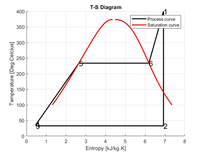
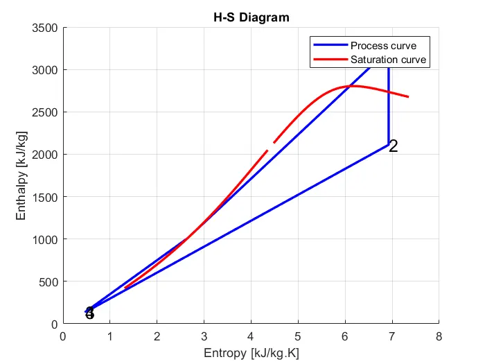
• To plot the corresponding T-s and h-s plots for the given set of inputs.

THEORY :

RANKINE CYCLE

The Rankine cycle is an idealized thermodynamic cycle describing the process by which certain heat engines, such as steam turbines or reciprocating steam engines, allow mechanical work to be extracted from a fluid as it moves between a heat source and heat sink. The Rankine cycle is named after William John Macquorn Rankine, a Scottish polymath professor at Glasgow University.

Heat energy is supplied to the system via a boiler where the working fluid (typically water) is converted to a high pressure gaseous state (steam) in order to turn a turbine. After passing over the turbine the fluid is allowed to condense back into a liquid state as waste heat energy is rejected before being returned to boiler, completing the cycle. Friction losses throughout the system are often neglected for the purpose of simplifying calculations as such losses are usually much less significant than thermodynamic losses, especially in larger systems.

EQUATIONS USED

Turbine work output (Wt) : H1 - H2

Pump work input (Wp) : H4 - H3

Net work done (W_net) : Wt-Wp

Heat input by the boiler (Q) : H1 - H4

Thermal Efficiency : (W_net / Q)*100

Specific Steam Consumpion (SSC) = 3600/W_net

Back work ratio = Wp/Wt

CODE :

clear all
close all
clc

%state variables at point 1
T1 = input('Enter the Temperature at the turbine inlet : ');  %to input temperature at point 1 (in degree celcius)
P1 = input('Enter the Pressure at the turbine inlet : ');     %to input pressure at point 1 (in Bar)
H1 = XSteam('h_pT',P1,T1);                                    %enthalpy in kJ/kg
S1 = XSteam('s_pT',P1,T1);                                    %entropy in kJ/kg.K

%state variables at point 2
P2 = input('Enter the Pressure at the condensor inlet : ');   %to input pressure at point 2
T2 = XSteam('Tsat_P',P2);                                  
S2 = S1;  

%finding dryness fraction
sf2 = XSteam('sL_p',P2);    
sg2 = XSteam('sV_p',P2);
hf2 = XSteam('hL_p',P2);
hg2 = XSteam('hV_p',P2);
x2 = ((S2-sf2)/(sg2-sf2));
H2 = hf2+(x2*(hg2-hf2));


%state variables at point 3
T3 = T2;
P3 = P2;
S3 = XSteam('sL_p',P3);
H3 = XSteam('hL_p',P3);
V3 = XSteam('vL_T',T3);


%state variables at point 4 
P4 = P1;
S4 = S3;

%finding Cp & Cv 
Cp = XSteam('Cp_ps',P4,S4);
Cv = XSteam('Cv_ps',P4,S4);
gamma = Cp/Cv;              %value for gamma
a = 1/gamma;
b = P3/P4;

%p3v3^gamma = p4v4^gamma
V4 = (b^a)*V3;              %volume at point 4
T4 = (P4*V4*T3)/(P3*V3);    %p4v4/T4 = p3v3/T3
H4 = XSteam('h_ps',P4,S4);

%state variables at point 5
P5 = P4;
T5 = XSteam('Tsat_p',P5);
S5 = XSteam('sL_p',P5);
H5 = XSteam('h_ps',P5,S5);

%state variables at point 6
P6 = P5;
T6 = XSteam('Tsat_p',P6);
S6 = XSteam('sV_p',P6);
H6 = XSteam('h_ps',P6,S6);

%system characteristics at given input conditions
W_output = H1-H2;                 %turbine work output
W_input = H4-H3;                  %turbine work input
W_net = W_output-W_input;         %net work
Q_input = H1-H4;                  %heat input given by the boiler
effi = (W_net/Q_input)*100;       %efficiency of rankine cycle
SSC = 3600/W_net;                 %specific steam consumption
B_work_ratio = W_input/W_output;  %back work ratio

%finding values of temperatures and entropies in saturation curve
t_curve = linspace(100,500,1000);         %assuming temperature varying from 100 to 500 in a sequence of 1000 even space
for i = 1 : length(t_curve);
    sL(i) = XSteam('sL_T',t_curve(i));    %entropy point in saturated liquid curve
    sV(i) = XSteam('sV_T',t_curve(i));    %entropy point in saturated vapour curve
    hL(i) = XSteam('hL_T',t_curve(i));    %enthalpy point in saturated liquid curve
    hV(i) = XSteam('hV_T',t_curve(i));    %enthalpy point in saturated vapour curve
end

%plotting T-S Diagram
figure(1)
hold on
plot([S1 S2 S3 S4 S5 S6 S1],[T1 T2 T3 T4 T5 T6 T1],'linewidth',2,'color','k') %plotting process curve
plot(sL,t_curve,'linewidth',2,'color','r')                                    %plotting saturation liquid curve
plot(sV,t_curve,'linewidth',2,'color','r')                                    %plotting saturation vapour curve
legend('Process curve','Saturation curve')                                    %legend
text(S1,T1,'1','fontsize',15)                                                 %numbering state points
text(S2,T2,'2','fontsize',15)
text(S3,T3,'3','fontsize',15)
text(S4,T4,'4','fontsize',15)
text(S5,T5,'5','fontsize',15)
text(S6,T6,'6','fontsize',15)
title('T-S Diagram')                %title of the plot
xlabel('Entropy [kJ/kg.K]')                   %naming x-axis
ylabel('Temperature [Deg Celcius]')               %naming y-axis
grid on                             %switching the grid


%plotting H-S Diagram
figure(2)
hold on
plot([S1 S2 S3 S4 S5 S1],[H1 H2 H3 H4 H5 H1],'linewidth',2,'color','b')  %plotting process curve
plot(sL,hL,'linewidth',2,'color','r')                                    %plotting saturation liquid curve
plot(sV,hV,'linewidth',2,'color','r')                                    %plotting saturation vapour curve
legend('Process curve','Saturation curve')                               %legend
text(S1,H1,'1','fontsize',15)                                            %numbering state points
text(S2,H2,'2','fontsize',15)
text(S3,H3,'3','fontsize',15)
text(S4,H4,'4','fontsize',15)
title('H-S Diagram')               %title of the plot
xlabel('Entropy [kJ/kg.K]')                  %naming x-axis
ylabel('Enthalpy [kJ/kg]')                 %naming y-axis
grid on                            %switching the grid

%printing processes
fprintf('\n(1-2) : Iscentropic expansion in Turbine \n')
fprintf('(2-3) : Constant pressure heat rejection inside Condeser \n')
fprintf('(3-4) : Iscentropic compression in Pump \n')
fprintf('(4-1) : Constant pressure heat addition inside Boiler \n')

%printing state variables at point 1
fprintf('\n At state point 1 : \n')
fprintf(' P1 is : %f Bar\n',P1)
fprintf(' T1 is : %f Deg Celcius\n',T1)
fprintf(' H1 is : %f kJ/kg\n',H1)
fprintf(' S1 is : %f kJ/kg.K\n',S1)

%printing state variables at point 2
fprintf('\n At state point 2 : \n')
fprintf(' P2 is : %f Bar\n',P2)
fprintf(' T2 is : %f Deg Celcius\n',T2)
fprintf(' H2 is : %f kJ/kg\n',H2)
fprintf(' S2 is : %f kJ/kg.K\n',S2)

%printing state variables at point 3
fprintf('\n At state point 3 : \n')
fprintf(' P3 is : %f Bar\n',P3)
fprintf(' T3 is : %f Deg Celcius\n',T3)
fprintf(' H3 is : %f kJ/kg\n',H3)
fprintf(' S3 is : %f kJ/kg.K\n',S3)

%printing state variables at point 4
fprintf('\n At state point 4 : \n')
fprintf(' P4 is : %f Bar\n',P4)
fprintf(' T4 is : %f Deg Celcius\n',T4)
fprintf(' H4 is : %f kJ/kg\n',H4)
fprintf(' S4 is : %f kJ/kg.K\n',S4)

%system characteristics at given input conditions
fprintf('\n System characteristics at given input conditions : \n')
fprintf(' Wt is : %f kJ/kg\n',W_output)
fprintf(' Wp is : %f kJ/kg\n',W_input)
fprintf(' Wnet is : %f kJ/kg\n',W_net)
fprintf(' Ntherm is : %f Percent\n',effi)
fprintf(' S.S.C is : %f kg/kWh\n',SSC)
fprintf(' Back work ratio is : %f',B_work_ratio)

INPUT :

Turbine Inlet temperature = 400° C

Turbine Inlet Pressure = 30 bars

Turbine Outlet Pressure = 0.05 bars = Condenser Inlet Pressure

OUTPUT :

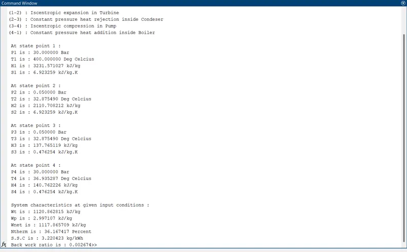
• Screenshot of command window showing the values of state variables and system characteristics w.r.t the input given.

• Temperature v/s Entropy Diagram of Rankine Cycle w.r.t the given input

• Enthalpy v/s Entropy Diagram of Rankine Cycle w.r.t the given input

EXPLANATION :

• Started the code by usual commands like clear all, close all and clc.
• In this program it's need to input some information to find the output, for that such information is assigned by "input" command as the user can input the necessary values while running, through command window.
• To find the desired values of enthalpy, entropy, temperature and pressure, used some commands to get the values from the "XSteam" file. For that the XSteam file should be saved in a folder where we saved the current program.
• After finding all values of each state points, find the work input, work output, heat input, thermal efficiency, specific steam consumption and back work ratio.
• "for loop" command is used to find the saturation curve for both T-S and H-S diagram by finding different entropy values w.r.t the temperature values which is defined by "linspace" command incase of T-S diagram and by finding different enthalpy values w.r.t the temperature incase of H-S diagram.
• Each values found are printed in the command window by "fprint" command.
• Plotted the graph T-S and H-S diagram by "plot" command by providing neccessary title, labels, legends and grid.
• "text" command is used to number the state points inside plot.

RESULT :

• Found the state variables like Temperature, Pressure, Enthalpy and Entropy of all state points.
• Found work done by the turbine which is equal to 1120.86 kJ/kg.
• Found work input to the pump which is equal to 2.997 kJ/kg.
• Found Net work done = 1117.86 kJ/kg.
• Found thermal efficiency which is equal to 36.167 %.
• Found Specific Steam Consumption which is equal to 3.22 kg/kWh.
• Found Back work ratio which is equal to 0.002674.