Week 3 - Solving second order ODEs

SOLVING SECOND ORDER ODE USING MATLAB

AIM:

To solve an Ordinary Differential Equation and to animate corresponding motion of Pendulum regarding the equation.

THEORY:

PENDULUM

A pendulum is a body suspended from a fixed point so that it can swing. The time interval of a pendulum’s complete back-and-forth movement is constant. There are several forces that acting on a pendulum in motion. The primary force is gravitational force which makes the back and forth motion of the pendulum and the centripetal force excerted by the spring which keep it moving in circular path in additional there may be some damping force which is due to the friction in the pivot or air resisitance or both.

ORDINARY DIFFERENTIAL EQUATION

An ordinary differential equation (ODE) is a differential equation containing one or more functions of one independent variable and the derivatives of those functions.

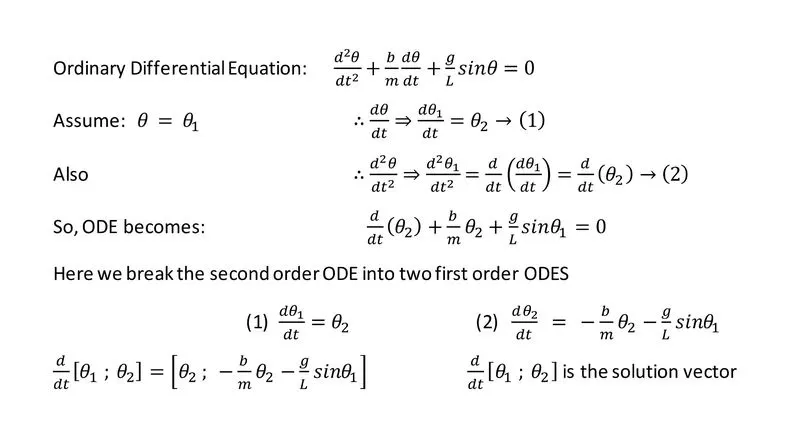
PROGRAM:

%function created to solve ODE

function [dtheta_dt] = ode_function(t,theta,b,g,l,m) 

theta1 = theta(1) 
theta2 = theta(2)
dtheta1_dt = theta2;
dtheta2_dt = -(b/m)*theta2-(g/l)*sin(theta1);
dtheta_dt = [dtheta1_dt ; dtheta2_dt];
end

%main program

clear all
close all
clc

b = 0.05; %damping coefficicent
g = 9.81; %gravity (m/s^2)
l = 1;    %Length of the spring (m)
m = 1;    %mass of the bob(Kg)

%initial condition
%angular displacement = 0
%angular velocity = 3 (m/s)
theta_0 = [0;3]; 

%time points
%pendulum oscillates between 0 - 20 seconds
%In a 80 evenly spaced sequence
t_span = linspace(0,20,800);

%solve ODE
[t,results] = ode45(@(t,theta) ode_function(t,theta,b,g,l,m),t_span,theta_0)

%plotting
figure(1)
plot(t,results(:,1))
hold on
plot(t,results(:,2))
title('Harmonic Motion of a Pendulum')
legend('Angular Displacement','Angular Velocity')
ylabel('Anugular Displacement and Velocity')
xlabel('time')
grid on

%for Loop
ct = 1 %counter value defined as 1
for i = 1 : length(results(:,1))
    theta = (results(i,1))
    
    x0 = 0
    y0 = 0
    
    x1 = l*sin(theta);
    y1 = -l*cos(theta);
    
    
    %plotting
    figure(2)
    plot([0 0],[0 1.5],'linewidth',10)
    hold on
    plot([x0 x1],[y0 y1],'linewidth',3)
    hold on
    plot(x0,y0,'marker','o','markersize',8,'markerfacecolor','y','markeredgecolor','r')
    plot(x1,y1,'marker','o','markersize',15,'markerfacecolor','g','markeredgecolor','r')
    hold off
    title('Motion of Pendulum')
    grid on
    axis([-1.5 1.5 -1.5 1.5])
    M(ct) = getframe(gcf);
    ct = ct+1 %In each iteration the counter value will increase by 1
end %end of for loop

%to create animation
movie(M) 
videofile = VideoWriter('motion of pendulum.avi','Uncompressed AVI')
open(videofile)
writeVideo(videofile,M)
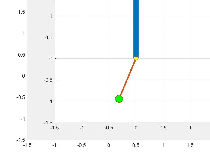
close(videofile)

OUTPUT: The animation video regarding the motion of pendulum has been shared via Youtube.

Youtube link : https://youtu.be/uWosoXzVGxs

EXPLANATION:

• Function regarding to solve the ordinary differential equation has been created in separate file. And this function will call while solving ODE.
• dtheta1_dt and dtheta2_dt are assigned with the corresponding values as shown in the equations.
• The file should save in a same name that of the function name.
• Then the main program is created in a separate file, started with clear all, close all and clc commands.
• The required inputs are introduced.
• The displacement and velocity are introduced in a column matrix form.
• The time of oscillation of the pendulum is introduced by 'linspace' command.
• Then 'ode45' an inbuilt function is used to solve the ODE while calling the function 'ode_func' which is created by us.
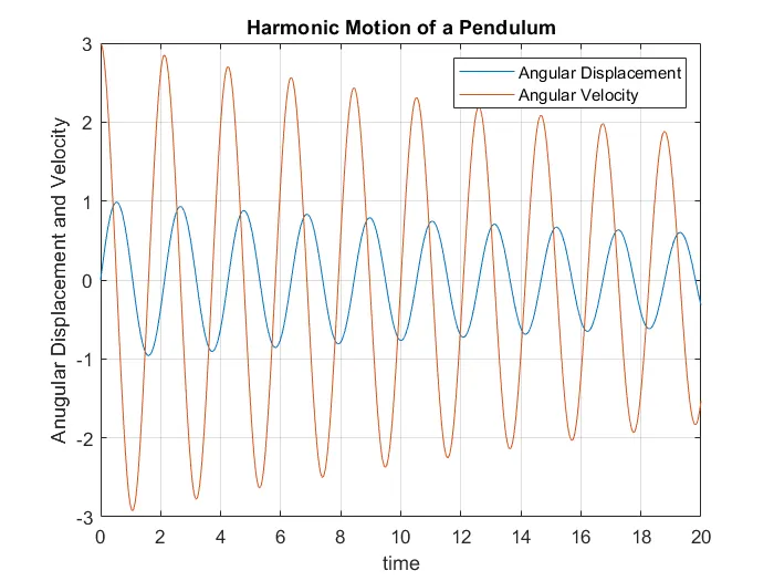
• The required plot regarding the changes occuring in Angular Displacement and Velocity has been created.
• A for loop has been introduced to get each position of the motion of pendulum.
• A variable has been introduced in a range from 1 to length of result 1 which is displacement.
• Then the end coordinate point of the pendulum are introduced.
• Then the required figure of pendulum is plotted.
• Then the each frame is stored in an array called 'M' which is therefore used to create animation.
• 'end' command is used to close the loop.
• After that the animation video is created.

CONCLUSION:

• The required curve of Angular Displacement and Angular Velocity has been plotted.
• The animation of motion of the pendulum has been created and shared via Youtube.