Week 4.1 - Genetic Algorithm

MAIN CODE: optimise the function and find the global maxima of the function

clear all 
close all
clc

% Input Paramters
x = linspace(0,0.5,150);
y = linspace(0,0.5,150);

% for number of Iterations
num_cases = 60;

% convert 1D to 2D array
[xx, yy] = meshgrid(x,y);

% Apply the for loop and apply the function of stalactite within formula 
tic
for i = 1:length(xx)
    for j = 1:length(yy)
   input_vector(1) = xx(i,j);
   input_vector(2) = yy(i,j);
   f(i,j) = stalactite(input_vector);
   end
end

%% Study 1 Unbounded
% By number of Iterations get the optimum values of x,y and f
for i = 1:num_cases
     % genetic algorithm for maximization
    [inputs, fopt(i)] = ga(@stalactite,2);
    xopt(i) = inputs(1);
    yopt(i) = inputs(2);
end
study_time = toc

%% Plotting of Study 1 Unbounded
figure(1)
subplot(2,1,1)
 surfc(xx,yy,-f)
 xlabel('x values')
 ylabel('y values')
 zlabel('Function Value')
 shading interp
 hold on
 title('Unbounded')

 % plot the optimum values of Study 1
 plot3(xopt,yopt,-fopt,'marker','o','markersize',5,'markerfacecolor','r')
 subplot(2,1,2)
 plot(-fopt)
 xlabel('Iterations')
 ylabel('Function maximum')
 
 %% study 2 Statistical behaviour within Upper and Lower Bounds
 % By number of Iterations get the optimum values within x and y lower and
 % upper limit
 tic
 for i= 1:num_cases
     [inputs, fopt(i)] = ga(@stalactite, 2,[],[],[],[],[0;0],[0.5;0.5]);
     xopt(i) = inputs(1);
     yopt(i) = inputs(2);
 end
 study_time2 = toc
 
 %% Plotting of Study 2 with lower and upper limits x and y 
 figure(2)
 subplot(2,1,1)
 surfc(xx,yy,-f)
 xlabel('x values')
 ylabel('y values')
 zlabel('Function Value')
 shading interp
 hold on
 
 % plot the optimum values of Study 2
 plot3(xopt,yopt,-fopt,'marker','o','markersize',5,'markerfacecolor','r')
 title('Bounded inputs')
 subplot(2,1,2)
 plot(-fopt)
 xlabel('Iterations')
 ylabel('Functions Maximum')
 
 %% study 3 Increasing the GA iterations
 
 % Increase the Number of genetic algorithm 
options  = optimoptions('ga')
 options = optimoptions(options,'PopulationSize', 150);
 
 % By number of Iterations get the optimum values within x and y lower and
 % upper limit and add options
 tic
 for i = 1:num_cases
     [inputs, fopt(i)] = ga(@stalactite, 2,[],[],[],[],[0;0],[0.5;0.5],[],options);
 xopt(i) = inputs(1);
 yopt(i) = inputs(2);
 end
 study_time3 = toc
 
 %% Plotting of Study 2 with lower and upper limits x and y 
 subplot(2,1,1)
 surfc(xx,yy,-f)
 xlabel('x values')
 ylabel('y values')
 zlabel('Function Value')
 shading interp
 hold on
 
 % plot the optimum values of Study 3
 plot3(xopt,yopt,-fopt,'marker','o','markersize',5,'markerfacecolor','g')
 title('Increased GA')
 subplot(2,1,2)
 plot(-fopt)
 xlabel('Iterations')
 ylabel('Function Maxima')
 

Explanation :

First of all, I defined the input variables x and y which will use in the curve equation. I define the limit of x and y from 0 to 0.5 and break it into 150 equal parts.

I defined the number of iterations (num_cases) as 60 to evaluate the f and fopt value 60 times .so the main objective is my f & fopt should be the same in every iteration.

Till this end, I have only 1-D array so I converted it into 2-D array by using meshgrid.

I applied the 'for loop' and measure the length of xx and yy 2-D array from starting line 1 and collect in i and j variables.

My maxima formula is 2 variable function, so I defined the variable named input_vector(1) and input_vector(2) which will act like input variables X and Y for the function value equation. that is equivalent to array xx containing i and j length.

Stalactite function for applying the mathematical 2 variable equation to get the maxima :

function [g] = stalactite(input_vector)
X1 = (sin(5.1*pi*input_vector(1)+0.5)).^6; 
X2 = exp(-4*log(2)*1.5625*(input_vector(1) - 0.0667).^2);
Y1 = (cos(5.1*pi*input_vector(2)+0.5)).^6;
Y2 = exp(-4*log(2)*1.5625*(input_vector(2) - 0.0667).^2);
g = -X1*Y1*X2*Y2;
end

Now, I defined the Variable f(i,j) and equate it to the stalactite function which is coded above and defined the equation of the curve.

% Study_1 Unbounded Statistical behaviour

According to the number of iterations I have to find the maximum function value in every iteration to 60. So I defined the variable -- (i) which is defined from 1 to num_cases.

Now, I defined the ga (General Algorithm) which is an inbuilt function and this will help in getting the minima value Which is containing my Stalactite function with 2 variables and Saving it in 2 variables named 'inputs' and 'fopt (optimum value of f)'. But I have to find the Global Maxima so I will change the positive to negative sign inside the stalactite function and my running main programing coding of maxima1. Then I will get the Global maxima instead of the minima.

'Inputs' has 2 columns and I split both columns into a different variable named xopt(i)--(optimum value of x and have 60 values of 60 Iterations) and yopt(i)--(optimum value of y and have 60 values of 60 Iterations) in inputs(1) and input(2).

%% plotting :

I took the subplot command and plot the 3D surface curve by using xx, yy (2D array value of x and y) and -f.

Now I plot the 3D point graph by xopt, yopt and -fopt to show the optimization results in points on the mountain's peak (maxima).

Now, I plotted the 2nd subplot command to show the plot between Function value and Iterations. According to the number of iterations Function value changes.

Here my 1st study is over.

%% study 2 Statistical behaviour within Upper and Lower Bounds :

In this study, I will apply the lower and upper limits for getting the nearly accurate values for optimization.

The coding for study 2 is the same as study 1 but the main difference is to apply the limit which is from 0 to 0.5 on the x and y-axis in the ga (genetic algorithm) in-built function.

%% study 3 Increasing the GA iterations :

The genetic algorithm starts with random samples, by default 'ga' took 60 samples of 2 variables so 60 sets of 2 Random variables, so it is population size. If the population size is too small then I will not find global maxima, but it will find local maxima.

So, I increased the population size to find the Global maxima.

----------------------------------------------------------------------------------------------------------------------------------------------------------------------------------------------------------------------------------------

Outputs:

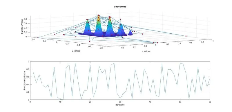
Study_1 Unbounded condition: I did not take the lower and upper limits for x and y. So optimum points (red) values of 'fopt' which value is generated by a genetic algorithm with stalactite function.

Study_2 Statistical behaviour with lower and upper limit bounds:

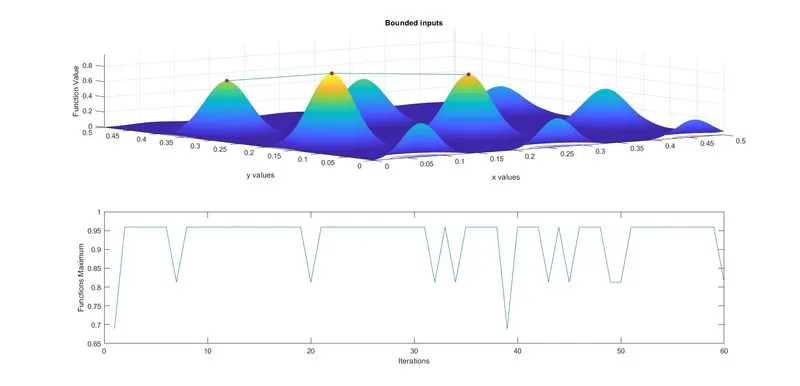
Here, I gave upper and lower limits of x and y which is giving a much narrow and accurate range of optimum value between 3 maxima peak points and variation of optimum values according to every Iteration is also much less.

Study_3 Increase the population size to get Global maxima:

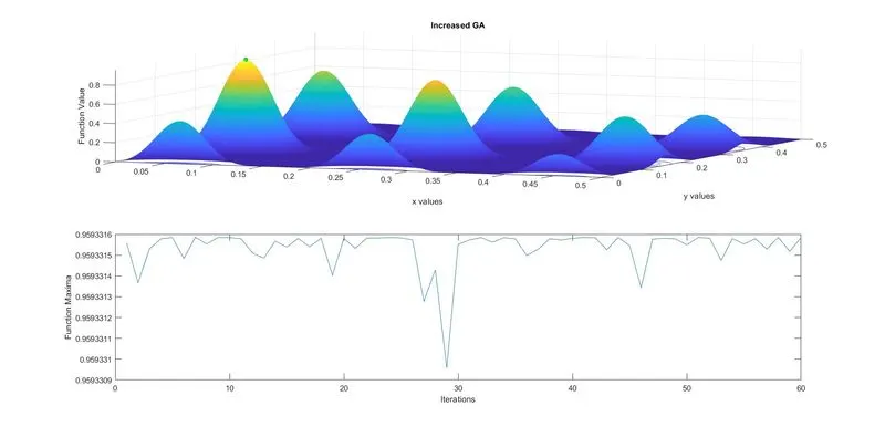
Here I took more population size which is nothing but 'ga' took 60 samples of 2 variables so 60 sets of 2 Random variables.

So I got the global maxima point (green) at the maximum height peak.

Now, I got a much more accurate Optimum value.

----------------------------------------------------------------------------------------------------------------------------------------------------------------------------------------------------------------------------------------

Problem during the programing for optimization(maxima) :

• Problem 1 = I am not getting the maximum points at the peak of mountains which is indicated with the red points (i.e data points).

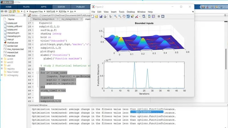
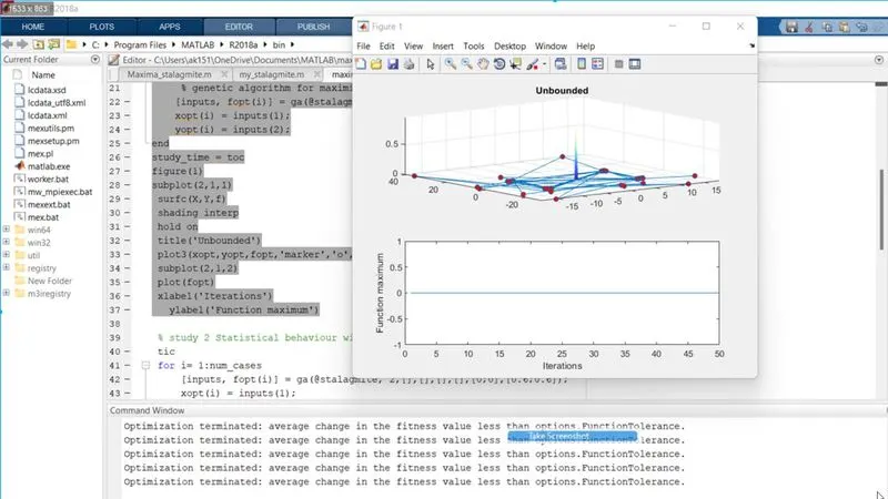
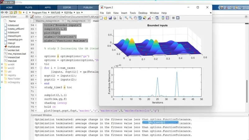
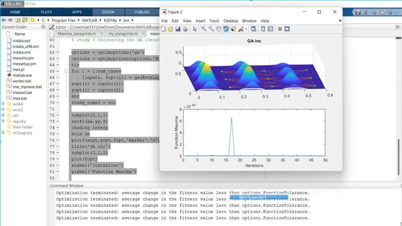
Solution : Because genetic algorithm (GA) gives always minima. But still I want to get the maxima value so I have changed the sign inside the stalactite function variable (g) so that the 3d plot can give the maxima value and red spot points on peaks to show the function maxima according to number of iteration.

function [g] = stalactite(input_vector)
X1 = (sin(5.1*pi*input_vector(1)+0.5)).^6;
X2 = exp(-4*log(2)*1.5625*(input_vector(1) - 0.0667).^2);
Y1 = (cos(5.1*pi*input_vector(2)+0.5)).^6;
Y2 = exp(-4*log(2)*1.5625*(input_vector(2) - 0.0667).^2);
g = -(X1*Y1*X2*Y2);
end

Now I will take the negative sign in the maxima1 (main) programing ;

figure(2)
subplot(2,1,1)
surfc(xx,yy,-f)
xlabel('x values')
ylabel('y values')
zlabel('Function Value')
shading interp
hold on

% plot the optimum values of Study 2
plot3(xopt,yopt,-fopt,'marker','o','markersize',5,'markerfacecolor','r')
title('Bounded inputs')
subplot(2,1,2)
plot(-fopt)
xlabel('Iterations')
ylabel('Functions Maximum')

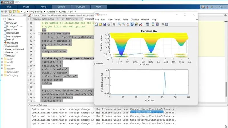
the sign inside the stalactite function variable (g) is positive so I got the minima value because GA gives a minima value.

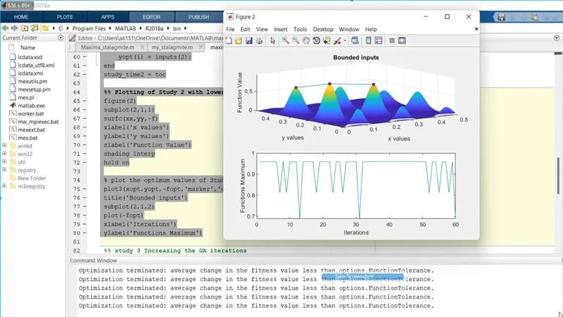
I changed the sign of the stalactite function variable (g) to negative so I got the maxima value and changed the sign of fopt, f. I got the mountain peak values.

---------------------------------------------------------------------------------------------------------------------------------------------------------------------------------------------------------------------------------------

Concept of genetic algorithm and explanation of the syntax for ga :

Genetic Algorithm (ga) is an inbuilt function in MatLab which is used to find the optimized (maxima/minima) value of the given problem in the form of the equation.

the syntax for ga is -- ga(@function, nvar, Aiq,Biq,Aeq,Beq,Lb,Ub,nonlcon,intcon,options)

Concept of genetic algorithm and explanation of the syntax for ga :

Genetic Algorithm (ga) is an inbuilt function in MatLab which is used to find the optimized (maxima/minima) value of the given problem in the form of the equation.

the syntax for ga is -- ga(@function, nvar, Aiq,Biq,Aeq,Beq,Lb,Ub,nonlcon,intcon,options)

function -- It contains the mathematical equations of a single or two variables by which I can find the maxima or minima value which can be useful.

nvar -- this shows how much the number of variables is present in the function's equation.

Aiq -- this shows the inequality relation equations in matrix form which is given by x, y and z constants of equations.

Biq -- this shows the inequality constants which are less than, greater than or equal to the equation of x, y and z variables equations.

Aeq -- this shows the equality relation equations in matrix form which is given by x, y and z constants of equations.

Beq -- this shows the equality constants which are equal to the equation of x, y and z variables equations.

Lb -- this shows the lower limits for x and y variables.

Ub -- this shows the Upper limits for x and y variables, these bounding conditions control the variation of optimum value in every iteration.

nonlcon -- this accepts the values of x and returns the C and Ceq vector. Which is representing the NON-LINEAR inequalities and equalities respectively.

intcon -- It takes the integer values which variable is listed in intcon.

options -- It minimize with the default optimization parameters replaced by value in options.