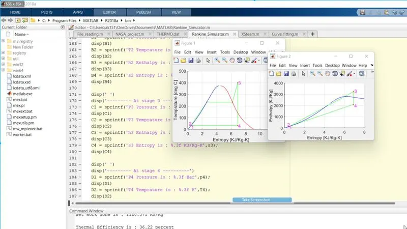
Project 2 - Rankine cycle Simulator
Main Programming for Rankine Simulator
clear all
close all
clc

disp('RANKINE SIMULATOR')
disp('PROCESS 1-2 ISENTROPIC EXPANSION IN PUMP')
disp('PROCESS 2-3 ISOBARIC HEAT ADDITION IN BOILER')
disp('PROCESS 3-4 ISENTROPIC EXPANSION IN TURBINE')
disp('PROCESS 4-1 ISOBARIC HEAT REJECTION IN CONDENSOR')
disp('INPUTS')

% Input Arguments (pressure in bar,temperature in deg celcius C)
p3 = 30
T3 = 400
p4 = 0.05

% /*Turbine Inlet*/ Superheated Steam
h3 = XSteam('h_pT',p3,T3);
s3 = XSteam('s_pT',p3,T3);

% /*Turbine Outlet*/ Steam with Dryness fraction
% h4 = hf+x*hfg
% s4 = sf4+x*sfg4

s4 = s3;
sf4 = XSteam('sL_p',p4);
sg4 = XSteam('sV_p',p4);

% Dryness Fraction
x = XSteam('x_ps',p4,s4);

h4 = XSteam('h_px',p4,x);
T4 = XSteam('T_ps',p4,s4);

% /*Pump Inlet*/saturated liquid
T1 = T4;
Tsat_1 = XSteam('Tsat_p',0.05);
s1 = XSteam('sL_T',Tsat_1);
h1 = XSteam('hL_T',Tsat_1);
p1 = XSteam('p_hs',h1,s1);

% /*Pump Outlet*/subcooled liquid
s2 = s1;
p2 = p3;
T2 = XSteam('T_ps',p2,s2);
h2 = XSteam('hL_T',T2);

Tsat2 = XSteam('Tsat_p',30);
psat2 = XSteam('psat_T',Tsat2);
ssat2 = XSteam('sL_T',Tsat2);
hsat2 = XSteam('hL_T',Tsat2);

Tsat3 = Tsat2;
ssat3 = XSteam('sV_T',Tsat3);

%% Saturation cuve (Dome)

T0 = linspace(0,500,500);

for i = 1:length(T0)
    Ssat_liquid_curve(i) = XSteam('sL_T',T0(i));
    Ssat_vapour_curve(i) = XSteam('sV_T',T0(i));

    Hsat_liquid_curve(i) = XSteam('hL_T',T0(i));
    Hsat_vapour_curve(i) = XSteam('hV_T',T0(i));
end

%% Plotting of T-S and H-S Diagram

% T-S Diagram
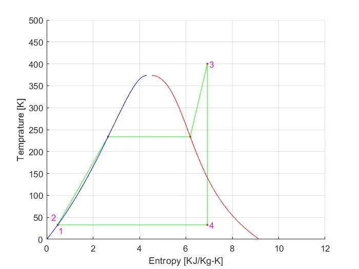
figure(1)
hold on
plot(s3,T3,'.','color','r')
plot(s4,T4,'.','color','r')
plot(s1,T1,'.','color','r')
plot(s2,T2,'.','color','r')
plot(ssat2,Tsat2,'.','color','r')
plot(ssat3,Tsat3,'.','color','r')
plot([s3 s4],[T3 T4],[s4 s1],[T4 T1],[s1 s2],[T1 T2],[s2 ssat2],[T2 Tsat2],[ssat2 ssat3],[Tsat2 Tsat3],[ssat3 s3],[Tsat3 T3],'color','g')
plot(Ssat_liquid_curve,T0,'color','b')
plot(Ssat_vapour_curve,T0,'color','r')
xlabel('Entropy [KJ/Kg-K]')
ylabel('Temprature [deg C]')
axis([0 12 0 500])
grid on

% Stages Indication
text(0.50,20,'1','color','m')
text(0.2,50,'2','color','m')
text(7,T3,'3','color','m')
text(7,T4,'4','color','m')

% H-S Diagram
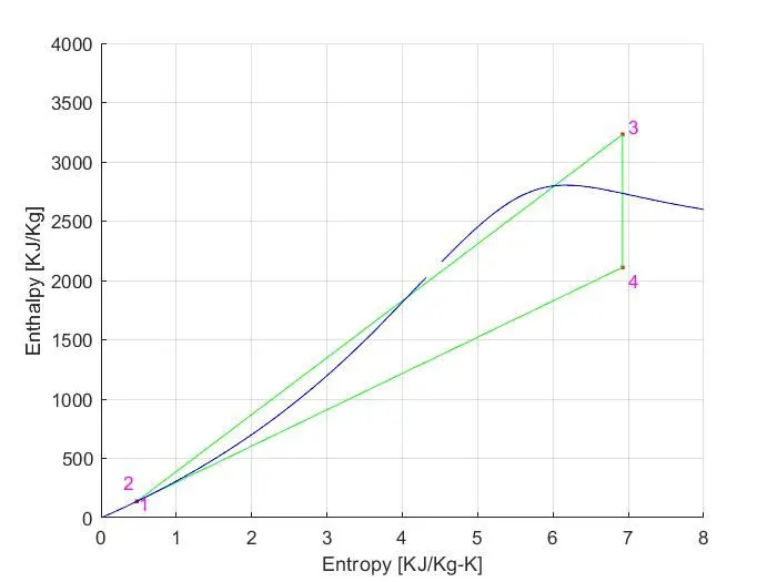
figure(2)
hold on
plot(s1,h1,'.','color','r')
plot(s2,h2,'.','color','r')
plot(s3,h3,'.','color','r')
plot(s4,h4,'.','color','r')
plot([s1 s2],[h1 h2],[s2 s3],[h2 h3],[s3 s4],[h3 h4],[s4 s1],[h4 h1],'color','g')
plot(Ssat_liquid_curve,Hsat_liquid_curve,'color','b')
plot(Ssat_vapour_curve,Hsat_vapour_curve,'color','b')
xlabel('Entropy [KJ/Kg-K]')
ylabel('Enthalpy [KJ/Kg]')
axis([0 8 0 4000])
grid on

text(0.50,120,'1','color','m')
text(0.3,300,'2','color','m')
text(7,3300,'3','color','m')
text(7,2000,'4','color','m')

%% Useful parameter calculations

% Heat Addition
Qadd = h3-h2;

% Heat Rejection
Qrej = h4-h1;

% Work done by the turbine
W_T = h3-h4;

%Work done on pump
W_P = h2-h1;

%Net Work done
Wnet = W_T-W_P;

% Thermal Efficiency (in % percent)

Th_eff = (Wnet/Qadd)*100;

% Specific Steam Consumption  (SSC) ( in Kg/(Kw-hr))
% Capicity of PowerPlant

SSC = 3600/Wnet;

%  Work Ratio
W_R = Wnet/W_T;

% Back work ratio
B_W_R = 1-W_R;

%% Show the Results in Command Window

disp('^_^ /*RESULTS*/ ^_^')

disp(' ')
disp('--------- At stage 1 ---------')
A1 = sprintf('P1 Pressure is : %.3f Bar',p1);
disp(A1)
A2 = sprintf('T1 Temprature is : %.3f K',T1);
disp(A2)
A3 = sprintf('h1 Enthalpy is : %.3f KJ/Kg',h1);
disp(A3)
A4 = sprintf('s1 Entropy is : %.3f KJ/Kg-K',s1);
disp(A4)

disp(' ')
disp('--------- At stage 2 ---------')
B1 = sprintf('P2 Pressure is : %.3f Bar',p2);
disp(B1)
B2 = sprintf('T2 Temprature is : %.3f K',T2);
disp(B2)
B3 = sprintf('h2 Enthalpy is : %.3f KJ/Kg',h2);
disp(B3)
B4 = sprintf('s2 Entropy is : %.3f KJ/Kg-K',s2);
disp(B4)

disp(' ')
disp('--------- At stage 3 ----------')
C1 = sprintf('P3 Pressure is : %.3f Bar',p3);
disp(C1)
C2 = sprintf('T3 Temprature is : %.3f K',T3);
disp(C2)
C3 = sprintf('h3 Enthalpy is : %.3f KJ/Kg',h3);
disp(C3)
C4 = sprintf('s3 Entropy is : %.3f KJ/Kg-K',s3);
disp(C4)

disp(' ')
disp('--------- At stage 4 ----------')
D1 = sprintf('P4 Pressure is : %.3f Bar',p4);
disp(D1)
D2 = sprintf('T4 Temprature is : %.3f K',T4);
disp(D2)
D3 = sprintf('h4 Enthalpy is : %.3f KJ/Kg',h4);
disp(D3)
D4 = sprintf('s4 Entropy is : %.3f KJ/Kg-K',s4);
disp(D4)

disp(' ')
disp('Results2')
E1 = sprintf('Heat Addition in boiler is : %.3f KJ/Kg',Qadd);
disp(E1)
E2 = sprintf('Heat Rejection in condensor is : %.3f KJ/Kg',Qrej);
disp(E2)

disp(' ')
E3 = sprintf('Work done by turbine is : %.3f KJ/Kg',W_T);
disp(E3)
E4 = sprintf('Work done on Pump is : %.3f KJ/Kg',W_P);
disp(E4)
E5 = sprintf('Net Work done is : %.3f KJ/Kg',Wnet);
disp(E5)

disp(' ')
E6 = sprintf('Thermal Efficiency is : %.2f percent',Th_eff);
disp(E6)

disp(' ')
E7 = sprintf('Specific Steam Consumption (SSC) is : %.3f Kg/(Kw-hr)',SSC);
disp(E7)

disp(' ')
E8 = sprintf('Back work ratio is : %.4f ',B_W_R);
disp(E8)
Explanation of Programming and Process of Rankine cycle
First of all, I displayed the main objective heading of the program which is the Rankine simulator. after that I displayed all process names of the Rankine cycle from point 1 to point 4.
% Inputs:
According to the Challenge question, I have to put the turbine Inlet pressure and temperature that is 400 deg Celsius and 30Bar so I used these parameters to find the Enthalpy, Entropy, Temperature and Pressure by Using the Steam table which is given by XSteam library. With the help of XSteam library, I can find the Saturation Curve with temperature, Entropy, Enthalpy and pressure.
% Calculation of Entropy, Enthalpy, Temperature and Pressure at every Stage Point:
I started from the Turbine inlet (stage 3) at this stage I found h3 (enthalpy) and s3 (entropy) from extracting the XSteam library. At this stage, water is in the form of Superheated Steam.
Now from stage 3 to stage 4 the Superheated Steam is Expanded isentropically and converted into semi vapour and liquid form( dryness fraction) at stage 4 .at this stage I calculated the enthalpy and Entropy and at this vapour form of water is entered into the condenser where heat is extracted isobarically from stage 4 to1 then vapour converted into saturated liquid form of water which is stage 1 and exit of condenser. So ,now from stage 1 to 2 the saturated liquid water is now isentropically expand into pump and entered into subcooled region , at stage 2 pump is increase the total Energy of water.
Now from stage 2 to 3 subcooled liquid is isobarically heated in boiler till superheated steam at stage 3 for achieving the dry steam.
% Dryness Fraction of Steam:
After the expansion of superheated steam dry vapour is converted into vapour+liquid form at the stage 4 so we have to calculate that what amount of liquid is present in steam.
so I used the XSteam library with x_ps now I have to put pressure and entropy value to get vapour fraction.
% How to draw saturation curve :
To draw the saturation curve I have to find all saturated states point of Entropy (S) and Enthalpy (H) with respect to the range value of temperature (0 to 500 deg C divided in 500 equal parts). Now,I used the for loop (i) to read the length of temperature range and apply in the Saturated liquid entropy(XSteam(sL_T,T(i))), Saturated vapour entropy(XSteam(sV_T,T(i))) and Saturated liquid enthalpy(XSteam(hL_T,T(i))), Saturated vapour enthalpy(XSteam(hV_T,T(i))). Now I got the all saturated value for Enthalpy(h) and Entropy(s) according to Ranged temperature.
Now, I plot Saturated liquid curve and Saturated vapour curve with respect to Temperature vs entropy graph and enthalpy vs entropy graph by using of plot(Ssat_liquid_curve,Hsat_liquid_curve,'color','b')
plot(Ssat_vapour_curve,Hsat_vapour_curve,'color','b').
%% Plotting of T-S and H-S diagram :
I used all 4 stages point of pressure, Enthalpy, Entropy and temperature and all saturated state point of Sat pressure, Sat Enthalpy, Sat Entropy and Sat temperature. now I got all stage point in one figure by hold on command. I used also the text command to show the stages 1,2,3 and 4.
%% Useful parameter calculation: Heat addition in boiler from stages 2 to 3 (Qadd = h2-h3). Work done by turbine (W_T = h3-h4). Heat rejection in condenser (Qrej = h4-h1). Work done on pump (W_P = h2-h1). Net work done (Wnet = W_T - W_P). Thermal Efficiency (in % ) Th_eff = (Wnet/Qadd)*100 Specific Steam Consumption (SSC) ( in Kg/(Kw-hr)) [Capicity of PowerPlant]SSC = 3600/Wnet.
Work Ratio W_R = Wnet/W_T . Back work ratio B_W_R = 1-W_R;
%% Show the Results in Command Window : For stage 1 ,I used variables A1,A2,A3 and A4 and equate them to sprintf to print the strings with respect to that stage properties variables like pressure, temperature, Entropy and Enthalpy etc after that I used the disp(A1) to display the values in command window. Similarly I used B,C,D and E variables in 4 counts. this method in all 4 stages to show the property in command window.
At last I have to show thermal efficiency ,Back work ratio ,Specific steam consumption(SSC), Net work done and Heat addition to boiler by using above method.
------------------------------------------------------------------------------------------------------------------------------------------------------------------------------------------------------------------------------------------
Output:
RANKINE SIMULATOR
PROCESS 1-2 ISENTROPIC EXPANSION IN PUMP
PROCESS 2-3 ISOBARIC HEAT ADDITION IN BOILER
PROCESS 3-4 ISENTROPIC EXPANSION IN TURBINE
PROCESS 4-1 ISOBARIC HEAT REJECTION IN CONDENSOR
INPUTS
p3 = 30 Bar
T3 = 400 deg C
p4 = 0.05 Bar
^_^ /*RESULTS*/ ^_^
--------- At stage 1 ---------
P1 Pressure is: 0.050 Bar
T1 Temperature is : 32.875 K
h1 Enthalpy is : 137.765 KJ/Kg
s1 Entropy is: 0.476 KJ/Kg-K
--------- At stage 2 ---------
P2 Pressure is: 30.000 Bar
T2 Temperature is : 32.945 K
h2 Enthalpy is : 138.056 KJ/Kg
s2 Entropy is: 0.476 KJ/Kg-K
--------- At stage 3 ----------
P3 Pressure is: 30.000 Bar
T3 Temperature is : 400.000 K
h3 Enthalpy is : 3231.571 KJ/Kg
s3 Entropy is : 6.923 KJ/Kg-K
--------- At stage 4 ----------
P4 Pressure is: 0.050 Bar
T4 Temperature is : 32.875 K
h4 Enthalpy is : 2110.708 KJ/Kg
s4 Entropy is: 6.923 KJ/Kg-K
Results2
Heat Addition in the boiler is: 3093.515 KJ/Kg
Heat Rejection in condenser is: 1972.943 KJ/Kg
Work done by the turbine is: 1120.863 KJ/Kg
Work done on Pump is : 0.291 KJ/Kg
Net Work done is : 1120.571 KJ/Kg
Thermal Efficiency is : 36.22 percent
Specific Steam Consumption (SSC) is : 3.213 Kg/(Kw-hr)
Back work ratio is : 0.0003
-------------------------------------------------------------------------------------------------------------------------------------------------------------------------------------------------------------------------------------------
Error while sketching the Saturated liquid-vapour curve
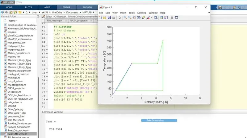
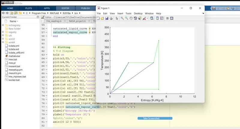
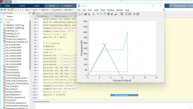
Solution : I used for loop with each and every value for Saturated liquid curve and saturated vapour curve
T0 = linspace(0,500,500)
for i = 1:length(T0)
Ssat_liquid_curve(i) = XSteam('sL_T',T0(i));
Ssat_vapour_curve(i) = XSteam('sV_T',T0(i));
Hsat_liquid_curve(i) = XSteam('hL_T',T0(i));
Hsat_vapour_curve(i) = XSteam('hV_T',T0(i));
end