Week 3 - Solving second order ODEs
CODE:
% solve the following Ordinary differential equation of the pendulum
% This ODE represents the equation of motion of a simple pendulum with damping

clear all
close all
clc

%% Input geometry parameters

% Length of pendulum (in meters)
L = 1;

% Mass of pendulum (in kg)
M = 1;

% Damping coefficient
C = 0.05;

% gravity (in m/s^2)
g = 9.81;

%% Initial Condition of Pendulum (at t = 0)

% motion study time (in second)
motion_time = linspace(0,20,620);

% Angular displacement (theta) and angular velocity (dtheta_dt)
theta_init = [0;3];

%% Solution of Ordinary differential equation

% Ordinary differential equation {d^2theta/dt^2 + (c/m)*dtheta/dt + (g/L)*sin(theta)} = 0 for simulating the pendulum

[t, y] = ode45(@(t,theta) ode_solver(t,theta,L,M,C,g),motion_time,theta_init);

%% Plotting and animating the pendulum (diagram 1)

figure(1)
ct=1;
for i = 1:length(y)
    theta_0 = y(i);

% Draw the string

% one end of string fix
x1 = 0;
y1 = 1;

% another end of string swimming

x2 = x1-L*sin(theta_0);
y2 = y1-L*cos(theta_0);

% Ball and string

plot([x1 x2],[y1 y2],[x1 x2],[y1 y2],'o','color','b');
xlabel('displacement in x direction')
ylabel('displacement in y direction')
axis([-1 1 -0.6 1])
pause(0.005)
OBS(ct) = getframe(gcf);
ct = ct+1;
end

% Create the movie
movie(OBS)
videofile = VideoWriter('pendulum_2.avi');
open(videofile)
writeVideo(videofile,OBS)
close(videofile)

%% plotting of displacement and velocity of a pendulum with respect to time (diagram 2)
figure(2)

plot(t,y(:,1))
hold on
plot(t,y(:,2))
xlabel('time')
ylabel('velocity (rad/s)(red curve) and displacement (rad)(blue curve)')
Explanation:
First of all, I have to define the all geometry parameters like string length (in meter), ball weight (in kg), gravity (m/s^2) and damping coefficient (c) etc.
Now, I have to define the initial state parameter of pendulum-like initial time =0, motion time = 20 seconds and divided into 1000 equal and for these 1000 parts the and displacement and angular velocity will break and these values increase and decrease with respect to the Ordinary differential equation which is dependent on time.
angular displacement(rad) and angular velocity (rad/sec) are 0 & 3 matrix form with theta_init. names are theta and dtheta_dt respectively. this angular displacement and angular velocity are changing with respect to time according to ODE so these can be converted into angular velocity and angular acceleration.
Now, I am going to use the Ordinary differential equation to solve the given pendulum problem {d^2theta/dt^2 + (c/m)*dtheta/dt + (g/L)*sin(theta)} = 0 by using the ode45 solver I will animate pendulum ball and string and I can show that in actual how the pendulum will act.
in the ode45 command, I gave that the whole equation is basically dependent on time and displacement angle theta and the whole equation is differentiated with respect to time.
the second term in ode45 is about solving the differential equation that what process and method is going on for solving the second-order equation of pendulum motion. the process /method was lengthy so I converted the method into the function and now I have to give the geometry parameter directly. the function for solving ODE is given below.
%% ODE solver:
function  [dtheta_dt] = ode_solver(t,theta,L,M,C,g)

% d^2theta/dt^2 + (C/M)*dtheta/dt + (g/L)*sin(theta) = 0

%For ease to solve ODE i will break into parts
 theta1 = theta(1)
 theta2 = theta(2)
 dtheta1_dt = theta2;
 dtheta2_dt = -(C/M)*theta2 - (g/L)*sin(theta1);
 dtheta_dt = [dtheta1_dt ; dtheta2_dt];
end
I wrote the general differential equation for a pendulum which is came from the Torque method from vibration.
From above for solving easy, I assumed theta1 = theta(1) and theta2 = theta(2) which is nothing but primary theta1 is used for velocity and for angular acceleration I will use differentiation of theta2 which is dependent on theta in theta1. so I mentioned separately theta 1 and theta2.
the dtheta1_dt is the rate change of displacement which is angular velocity and we got the middle differential term of the equation equal to theta2.
dtheta2_dt is the rate change of angular velocity which is angular acceleration and we got the first differential term of the equation equal to
-(C/M)*theta2 - (g/L)*sin(theta1) directly from general equation. now i have to put the constant value from main program t,theta,L,M,C,g.
function over...
In the main programming, the next terms are motion_time and theta_init of the ode45 function which are already defined.
From ode45, I will find the vector [t, y] .t contains the time from 0 to 20 in 1000 parts and y contains 2 columns of 1000 rows, the first column is contained 1000 rows of displacement and the second column is contained 1000 row of velocity which both columns value are increasing and decreasing with respect to time.
%% Plotting and animating the pendulum (diagram 1):
In the plotting section, I will show the 2 plots in which one plot will show the animation of the pendulum and how the pendulum is swimming according to the variable y and the second plot will show the graph of displacement and velocity which is dependent on time.
Now I have started the code for animating the pendulum for which I will put the name figure(1).
Apply the (for) Loop to repeat the oscillation of the pendulum for 20 seconds. I know the length of variable y is 1000 according to the part of time .so I defined the i = 1: length(y) so that the value can read from 1 to 1000 of (y).
Now I can change the angular displacement according to time which is already saved in (y).
But for ease of running and coding, let theta_0 = y(i) and this variable will be used for the motion of the pendulum which will join from another end of the string.
For drawing the string, I fixed the one end from the top which is according to coordinate means x1 = 0 and y1 = 1.
Now I have to define another coordinate for the end of the string which is free and ready for swimming according to variable y (displacement and velocity 1000 values).
coordinates for end of string are x2 = x1-L*sin(theta_0); y2 = y1-L*cos(theta_0); x-coordinate is function of sin(theta_0) which value will change 1000 times and subtract from x1.so in x axis pendulum will oscillate.
y-coordinate is a function of cos(theta_0) and this value will change 1000 times and subtract from y1. so in y-axis pendulum will oscillate. In this way, I defined the coordinate for the pendulum string and ball.
Now I used the plot command for sketching the string and pendulum ball together. I named the x-axis x displacement and y-axis y displacement.
For Fixing the plot x-axis and y-axis, I will use the axis command so that it can not vary according to the variation of the pendulum and defined the fixed axis's values.
For visible animation of the pendulum diagram, I will use the pause command with a 0.005 value and apply the end to finish the (for) Loop command.
%% plotting of displacement and velocity of a pendulum with respect to time (diagram 2):
I named the second plot figure(2) which is opened after the ending of the animation of the pendulum and shows the velocity, and displacement with respect to time.
Already I have solved the ODE and get matrix [t, y] which contains time, displacement and velocity. In the first plot command, the graph will draw between displacement and time and in the second plot command, the graph will draw between velocity and time. I used the hold on command so that both graphs can show in one figure(2). I named x and y-axis time and velocity (rad/s)(red curve) and displacement (rad)(blue curve) respectively.
At last, I will create a movie for saving the animation of the pendulum.
-----------------------------------------------------------------------------------------------------------------------------------------------------------------------------------------------------------------------------------------------------------------------
Output:
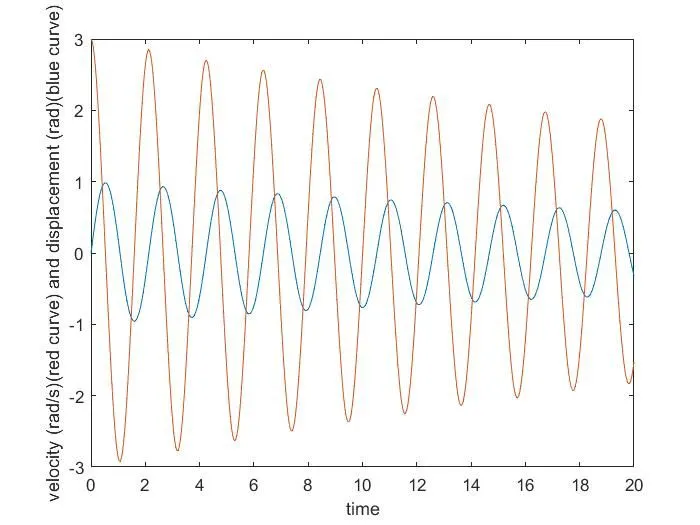
Explain : Explain: y term contains 2 values (column 1) displacement and (column 2) velocity which are varying with time according to solving the differential equation. I used the (:,1) so that the first column of y variable of the first column to its length read and plot it then and use the (:,2) so that the second column of y variable to its length read and plot it between velocity and time and hold on.
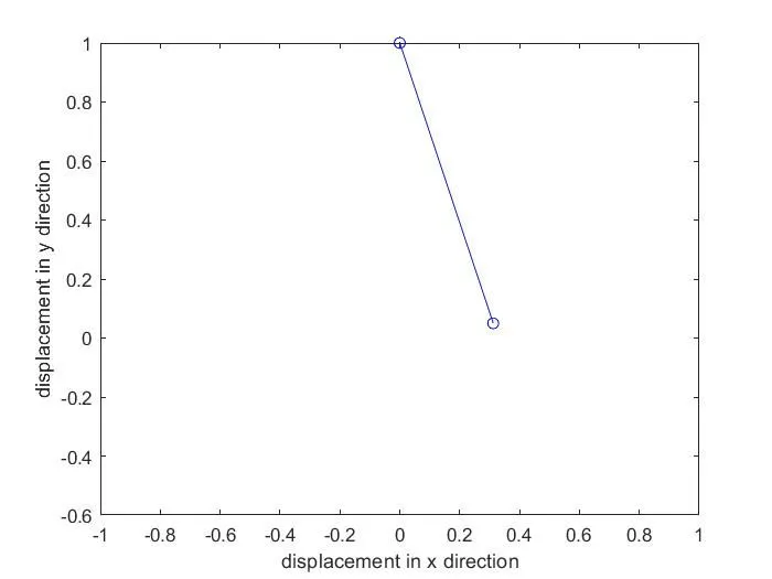
Animation: https://www.youtube.com/watch?v=EdOJLCRvSVk
Uncompressed avi is taking 650MB so I will only use the pendulum_2.avi command, please turn off the Ransomware protection to get the animation.
I used OBS instead of M because M was not allowed to make animation.
The pendulum ball is displacing in x and y directions according to x2 = x1-L*sin(theta_0) y2 = y1-L*cos(theta_0);
---------------------------------------------------------------------------------------------------------------------------------------------------------------------------------------------------------------------------------------------------------------------
Problems during the writing and simulating the program for Pendulum by Ordinary differential equation of Pendulum with Solution :
Problem 1: I am facing the challenge to write the ODE means ode45 command to study the motion of a pendulum. I wrote that the equation dependent on theta (displacement) and time but unable to apply the full statement.
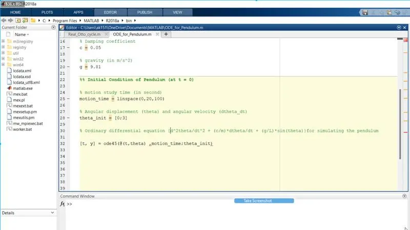
Solution: I have made a function named ode_solver in which the differential equation is solved for particular this case.
Problem 2: I tried to draw the string and animate it by giving the coordinate
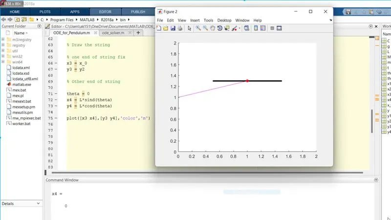
Solution: I erase the sin and cos in degree and put only sin and cos terms because approx. everything is going on the rad.
Problem 3: I have traced but am unable to make it correct like the string
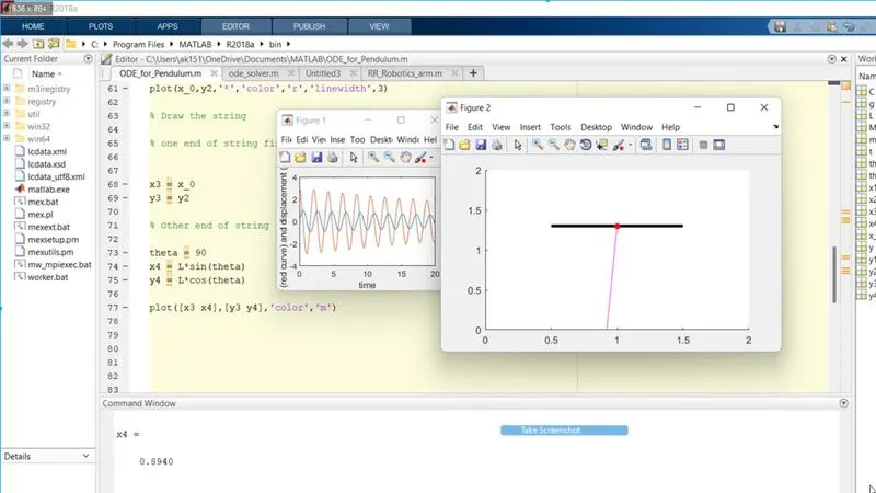
Solution: now I used the for loop for angle increment and pause for animate.
Problem 4: but animate is again now incorrect, it should be according to ODE.
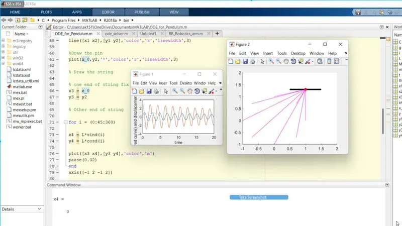
Solution: I used the i = 1: length(y) and theta_0 = y(i) so that the theta_0 can access the 1000 value of y (contains displacement and velocity) and apply for free end of string/pendulum.
Problem 5: Now my animation is working but still it is animating the wrong pattern according to ODE and it is overwriting in figure 1 also
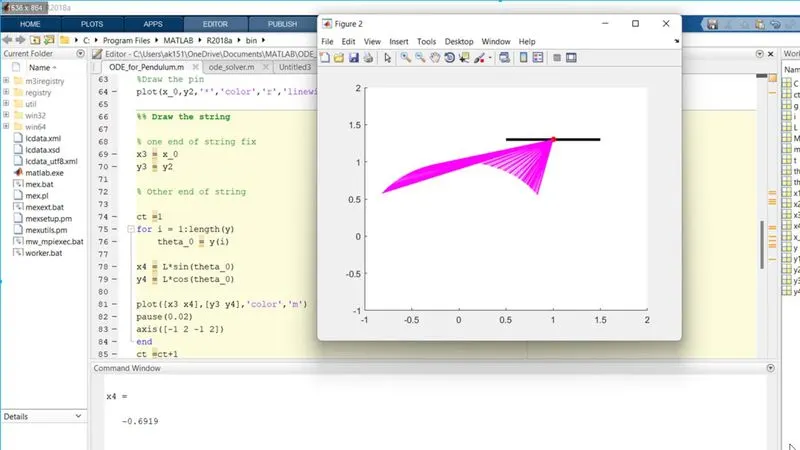
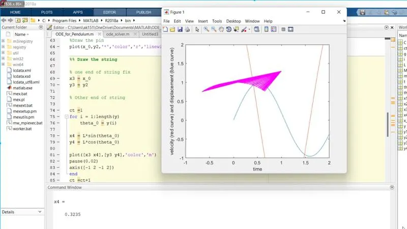
Solution: Firstly, I executed the pendulum oscillation figure after that I executed the plot command to sketch the plot between, displacement, and velocity with respect to time. Otherwise 'hold on' command will work on both figures which will lead to the overwritten plot.
Problem 6: Incorrect tracing of the path by the pendulum.
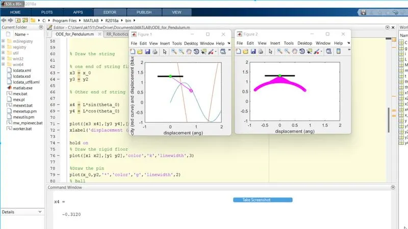
Solution: Now have changed the free side string end equation of position of different values of displacement i.e. x4 = x3-L*sin(theta_0) , y4 = y3-L*cos(theta_0) and many plot command eliminated, string and marker only left on plot.
Problem 7: But still my animation is not correct, figure 2 is overwritten in figure 1
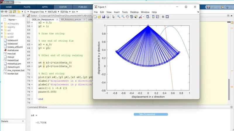
Solution: Firstly, I executed the pendulum oscillation figure after that I executed the plot command to sketch the plot between, displacement, and velocity with respect to time. Otherwise 'hold on' command will work on both figure which will lead to overwrite plot
Problem 8: Error message in command window during the creation of the movie.
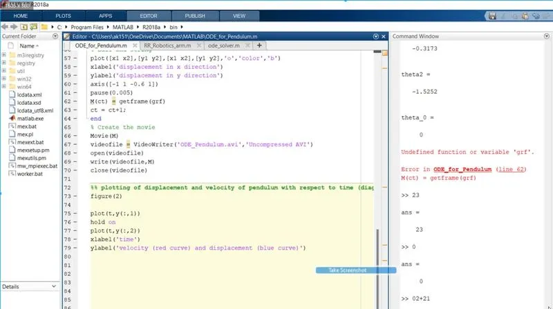
Solution: for making a movie used the OBS instead of M and my video gets ready.