Week 4.1 - Genetic Algorithm

AIM : To write a matlab code to optimize the stalegmite function & find the global maxima of the function.

Here in there is the term optimization is used lets understand it in a bit detail.

Optimization :

Optimization is the the action of making the best or most effective use of a situation or resource.

In every process there are set of inputs & outputs. Optimizing refers to finding the values of the inputs in such a way so that we can get the best output values.

Optimization techniques are the techniques used to discover the best solution out of all the possible solutions available under the constraints present. The genetic algorithm is one such optimization algorithm built based on the natural evolutionary process of our nature. The idea of Natural Selection and Genetic Inheritance is used here. Unlike other algorithms, it uses guided random search, i.e., finding the optimal solution by starting with a random initial cost function and then searching only in the space with the least cost (in the guided direction). Suitable when you are working with huge and complex datasets.

Now lets have a bit more detailde idea regarding genetic algorithm.

Genetic Algorithm :

The genetic algorithm developed by John Holland and his collaborators in the 1960s and 1970s (Holland, 1975; De Jong, 1975), is a model or abstraction of biological evolution based on Charles Darwin's theory of natural selection. Holland was probably the first to use the crossover and recombination, mutation, and selection in the study of adaptive and artificial systems. These genetic operators form the essential part of the genetic algorithm as a problem-solving strategy. Since then, many variants of genetic algorithms have been developed and applied to a wide range of optimization problems, from graph coloring to pattern recognition, from discrete systems (such as the travelling salesman problem) to continuous systems (e.g., the efficient design of airfoil in aerospace engineering), and from financial markets to multi-objective engineering optimization.

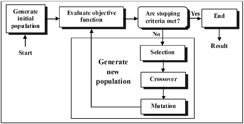
As we have seen in the above description there are three main components or genetic operators in genetic algorithms which are,

1) Crossover

2) Mutation

3) Selection of the fittest

The genetic algorithm is based on the genetic structure and behavior of the chromosome of the population. The following things are the foundation of genetic algorithms.

• Each chromosome indicates a possible solution. Thus the population is a collection of chromosomes.
• A fitness function characterizes each individual in the population. Therefore, greater fitness better is the solution.
• Out of the available individuals in the population, the best individuals are used to reproduce the next generation offsprings.
• The offspring produced will have features of both the parents and is a result of mutation. A mutation is a small change in the gene structure.

Basic Strucuture of Genetic Algorithm :

Now lets look at its advantages & limitations.

Advantages :

• It does not require any derivative information.
• It do have very good parallel capabilities.
• As compared to Traditional methods it is much more faster & efficient.
• It just not provide a single solution but the list of good solutions.
• It always gets an answer for the problem & which gets better over the time.
• It is very useful when the search space is very large & also when there are large number of parameters involved.

Limitations :

• Genetic A;gorithm is not suited for all kinds of problems especially problems which are simple & for which derivative information is available.
• Fitness value is calculated repeatedly which might be computationally expensive for some problems.
• Being stochastic , there are no guarantees on the optimality or the quality of the solution.
• Improper implementation of GA may not converge to the optimum solution.

Applications :

1. Acoustics :-

GA is used to distinguish between sonar reflections and different types of object. Apart from that it is also used to design Active noise control systems which cancel out undesired sound by producing sound waves that destructively interfere the unwanted noise.

2. Aerospace Engineering :-

To design wing shape Super Sonic aircraft minimizing aerodynamic drag at supersonic cruising speeds, minimizing drag at subsonic speeds, and minimizing aerodynamic load .

3. Financial Markets :-

to predict the future performance of publicly traded stocks.

4. Geophysics :-

locate earthquake hypo centers based on seismological data.

5. Materials Engineering :-

To design electrically conductive carbon based polymers known as polyanilines. To design exposure pattern for an electron lithography beam.

6. Routing and Scheduling :-

To find optimal routing paths in telecommunication networks which are used to relay data from sender to recipients .

7. Systems Engineering :-

To perform multi–objective task of designing wind turbines used to generate electric power.

8. Data mining :-

GA can also be used in data mining and pattern recognition. Given a large set of data, GA can perform a search for the optimum set of data which satisfies the conditions. Initial population in this case may be single objective conditions and at the end of the GA, we get a combined complex condition which when applied on the large data set can lead to finding the required set of data.

Syntax for ga :

Lets consider below 3 scenarios.

1) x = ga(fitnessfcn,nvars)

The above condition finds a local unconstrained minimum x.

Here fitnessfcn is the objective function &

nvars is the dimension of fitnessfcn.

2) x = ga(fitnessfcn,nvars,A,b,Aeq,Beq,LB,UB)

The above condition defines a set of lower & upper bounds on the design variable x, so that the solution can be found out within the range LB≤x≤UB.

Do set Aeq=[] & Beq=[] if no linear equalities exist.

3) x = ga(fitnessfcn,nvars,A,b,Aeq,Beq,LB,UB,nonlcon,option)

The above condition minimizes with the default optimization parameters replaced by values in options.

Create options using optimoptions or gaoptimset.

Now lets proceed further towards coding to find the global maxima with the use of genetic algorithm.

Function of stalegmite can be defined as given below.

f(x,y) = f1x.f1y.f2x.f2y

f1x = (sin(5.1πx+0.5))^6

f2y = (sin(5.1πy+0.5))^6

f2x = exp[-4ln(2).((x-0.667)^2/0.64)]

f2y = exp[-4ln(2).((y-0.667)^2/0.64)]

Stalegmite Function Program :

%Creating stalagmite function

function f = stalagmite(input_vector)

%selected two variables x & y for the function

x = input_vector(1);
y = input_vector(2);

f1x = (sin(5.1*pi*x+0.5))^6;
f1y = (sin(5.1*pi*y+0.5))^6;

f2x = exp(-4*log(2)*((x-0.0667)^2)/0.64);
f2y = exp(-4*log(2)*((y-0.0667)^2)/0.64);

% Minus sign denotes inverse of stalegmite function & this minus sign is added to get the maximum value as GA algorithm always gives the minimum value. 

f = -(f1x*f1y*f2x*f2y);

end

Study-1 :

Here the first study concerns with the unbounded inputs provided for calculating the value of global maxima.

Program-1 :

clear all
close all
clc

%Defining the search space
x = linspace(0,0.6,150);
y = linspace(0,0.6,150);

%Counting Iteration
num_cases = 400;

%Creating a 2D Mesh
[xx , yy] = meshgrid(x,y);

%Eveluating the stalagmite function
for i = 1:length(xx)
for j = 1:length(yy)
input_vector(1) = xx(i,j);
input_vector(2) = yy(i,j);
f(i,j) = stalagmite(input_vector);
end
end

for i = 1:num_cases
[inputs, fval(i)] = ga(@stalagmite,2);
opt_x(i) = inputs(1);
opt_y(i) = inputs(2);
end

figure(1)
subplot(2,1,1)
surfc(xx,yy,-f)
hold on

%Removing gridlines on the 3D surface plate for smoother appearance of the surface
shading interp

plot3(opt_x,opt_y,-fval,'marker','*','markersize',2)
title('Unbounded Inputs')
subplot(2,1,2)
plot(-fval)
xlabel('Total Iterations')
ylabel('Fmax')

Result :

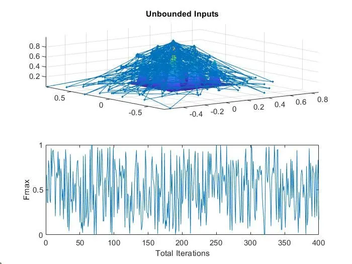
The results obtained in the unbounded inputs vary over a large sized interval.Due to that it provides unclear idea of the global maxima. But the value of Fmax can be observed between the interval [0,1]. So that for the precise results we should opt for bounded inputs.

Study-2 :

The second study is concerned with the bounded inputs provided for calculating the value of global maxima.

Program-2 :

clear all
close all
clc

%Defining the search space
x = linspace(0,0.6,150);
y = linspace(0,0.6,150);

%Counting Iteration
num_cases = 400;

%Creating a 2D Mesh
[xx , yy] = meshgrid(x,y);

%Eveluating the stalagmite function
for i = 1:length(xx)
for j = 1:length(yy)
input_vector(1) = xx(i,j);
input_vector(2) = yy(i,j);
f(i,j) = stalagmite(input_vector);
end
end

%programming for bounded inputs
for i = 1:num_cases
[inputs, fval(i)] = ga(@stalagmite,2,[],[],[],[],[0;0],[1;1]);
opt_x(i) = inputs(1);
opt_y(i) = inputs(2);
end

figure(2)
subplot(2,1,1)
surfc(xx,yy,-f)
xlabel('x value')
ylabel('y value')
hold on
shading interp
plot3(opt_x,opt_y,-fval,'markersize',2)
title('Bounded Inputs')
subplot(2,1,2)
plot(-fval)
xlabel('Total Iterations')
ylabel('Fmax')

Result :

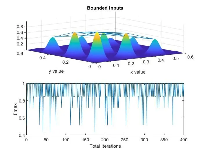
From the above resulting plot, we can understand that the value of global maxima lies in between the interval [0.8,1]. To get the better idea we can specify Population size that can justify our results & provide us with the near to exact solution.

Study-3 :

Third study is concerned with the bounded inputs provided but with a varies population size for better optimization in order to calculate the value of global maxima.

Program-3 :

clear all
close all
clc

%Defining the search space
x = linspace(0,0.6,150);
y = linspace(0,0.6,150);

%Counting Iteration
num_cases = 400;

%Creating a 2D Mesh
[xx , yy] = meshgrid(x,y);

%Eveluating the stalagmite function
for i = 1:length(xx)
for j = 1:length(yy)
input_vector(1) = xx(i,j);
input_vector(2) = yy(i,j);
f(i,j) = stalagmite(input_vector);
end
end

%Programming for bounded inputs with altered population size
options = optimoptions('ga');
options = optimoptions(options,'Populationsize',600);

for i = 1:num_cases
[inputs, fval(i)] = ga(@stalagmite,2,[],[],[],[],[0;0],[1;1],[],[],options)
opt_x(i) = inputs(1);
opt_y(i) = inputs(2);
end

figure(3)
subplot(2,1,1)
surfc(xx,yy,-f)
xlabel('x value')
ylabel('y value')
hold on
shading interp
plot3(opt_x,opt_y,-fval,'marker','*','markersize',2)
title('Bounded inputs with altered population size')
subplot(2,1,2)
plot(-fval)
xlabel('Total Iterations')
ylabel('Fmax')

Result :

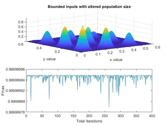
Use of population method within the bounded inputs increases the probability of determining the exact value of global maxima. Here, assumed value of population size is 600.

Explaination of the Program :

1. The stalagmite function was initially mentined with the appropriate argument vectors.
2. The program has been subdivided into the three studies based on the limitations of the previous study for the improvement & to finally get the exact solution.
3. First study deals with the unbounded inputs, so expanding the boundary wherein the results can be obtained.
4. Second study brings in the aspect of bounded inputs providing a better solution for the drawback faced.
5. The third study provides the appropriate platform to get the exact solution.
6. Plots of all the studies are provided below their programs to get the clear ideaof the results.

Error faced during programing :

During programing minus sign was inserted in the program by mistake so got the error in command window as shown in the image.

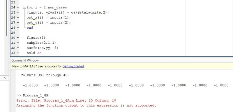
Solution :

Minus sign was removed to solve the error & after that the program ran fine.