Week 4.1 - Genetic Algorithm
AIM:
To optimize the stalagmite function using genetic algorithm techniques using MATLAB.
To understand the genetic algorithm first, we need to understand the following concepts to build a basic understanding of the genetic algorithm.
STALAGMITE:
A stalagmite is an upward-growing mound of mineral deposits that have precipitated from water dripping onto the floor of a cave. Most stalagmites have rounded or flattened tips. There are many other types of mineral formations found in caves.
LOCAL AND GLOBAL OPTIMA:
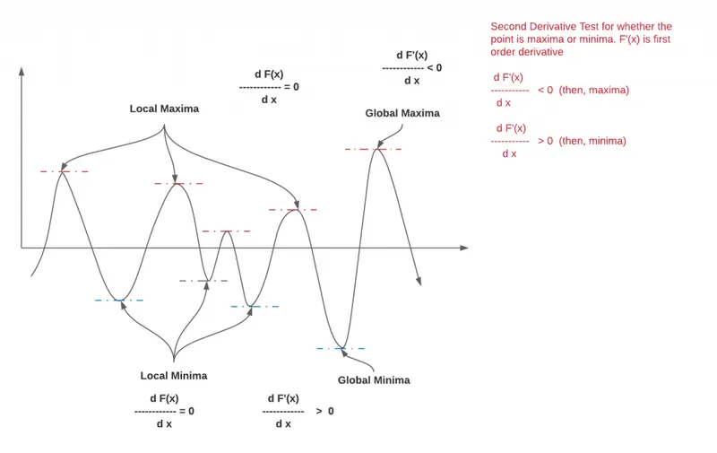
A local minimum of a function is a point where the function value is smaller than at nearby points, but possibly greater than at a distant point. A global minimum is a point where the function value is smaller than at all other feasible points.
OPTIMIZATION:
Optimization is the process of making something better (such as adesign, system, or decision) as fully perfect functional, or effective as possible, this also helps us to find the best possible results under a set of constraints. This process is excecuted again and again till the result or the output is satisfactory. This includes maximizing the product, strength, reliability, efficiency, and utilization.
Example- Taking the design of a wing of an aircraft, handling a load of 1 tonne what considerations are to be chosen as parameters? Length, width,(aspect ratio) the factor of safety, weight, and stress-induced, etc. So choosing the factor of safety and stress-induced over the beam is within limits.
various optimization techniques that can be used to optimize the result.
Determinstic method: In this method, the output of the model is fully determine by the parameter of the initial conditions. This uses specific rules from moving from one solution to another. let us understand with the help of an example:
stress analysis of wing is determined as the output result(stress value) is totally dependent on the initial condition (loading condition) and the parameters like material and forces acting on the component.
Stochastic Algorithms: The stochastic algorithms are in nature with probabilistic translation rules. These are gaining popularity due to certain properties which deterministic algorithms do not have.
This method is used for minizing and maximizing an objective function, this possesses some inherent randomness, it is probabilistic approach. This method is gaining popularity due to some properties which deterministic method does not possess. let us understand with an example imagine a company that provides energy to household based on how much they demand.
The following is the procedure followed by an optimization process.
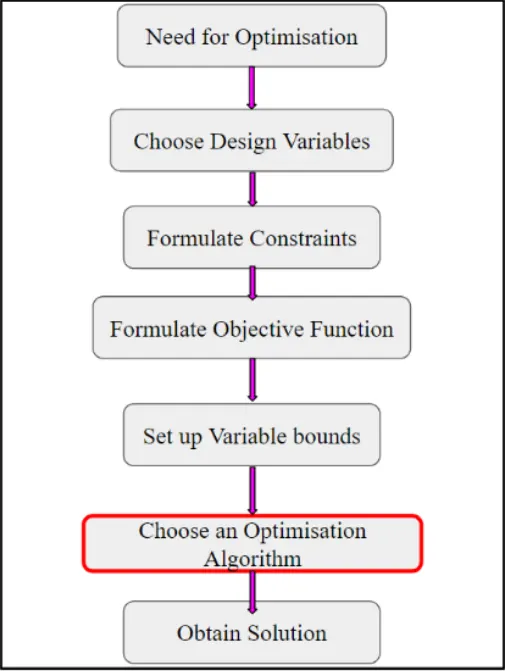
Variables- Variables is a pocess that may vary during optimization is my variables. An example is the dimension of a design that can be scale-up or vary to get minimum stress.
Constraints- During the optimization your output must not go beyond certain limits are known as constraints. An example one can reduce the material in such a way that the stress must not exit the ultimate stress of the material.
Objective function- This can be predicted by the mathematical model that includes all the variables as input. for example z=(x,y) here the z output is totally dependent on the input variable (x,y).
Variable bound- These are the range of the variable input, that will be varied at every iteration to provide an optimized result. For example, the desgin variable can be varied in between the set of a range to get the minimum stress.
The concept of Genetic Algorithm
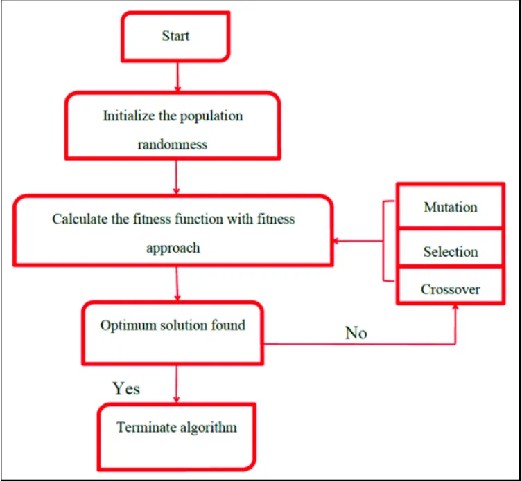
A genetic algorithm is a natural process that is used for the selection of the fittest individuals. The main use of the genetic algorithm is for reproduction to produce offspring of the next generation, this process of selecting and reproducing the fittest individual is inspired by Charles Darwn's and named it the "Theory of evolution".
Notion of Natural Selection
The process of natural selection starts with the selection of fittest individuals from a population. They produce offspring which inherit the characteristics of the parents and will be added to the next generation. If parents have better fitness, their offspring will be better than parents and have a better chance at surviving. This process keeps on iterating and at the end, a generation with the fittest individuals will be found.
This notion can be applied for a search problem. We consider a set of solutions for a problem and select the set of best ones out of them.
Five phases are considered in a genetic algorithm.
- Initial population
- Fitness function
- Selection
- Crossover
- Mutation
Initial Population
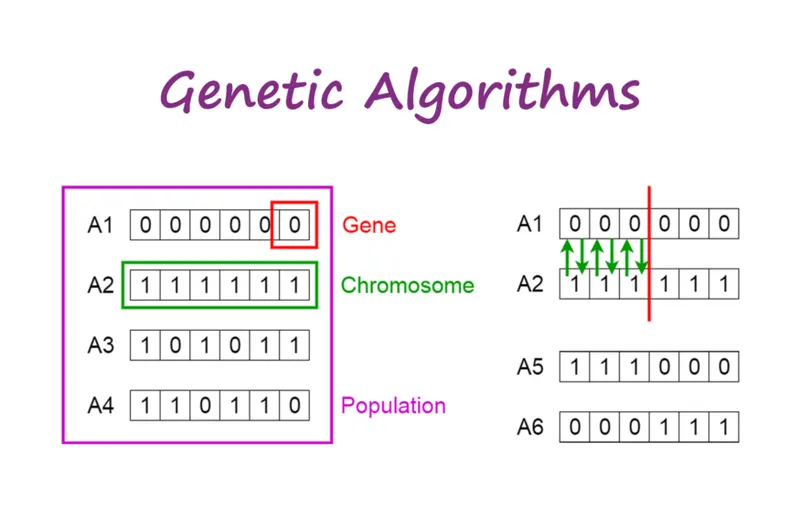
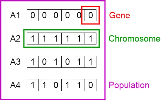
The process begins with a set of individuals which is called a Population. Each individual is a solution to the problem you want to solve.
An individual is characterized by a set of parameters (variables) known as Genes. Genes are joined into a string to form a Chromosome (solution).
In a genetic algorithm, the set of genes of an individual is represented using a string, in terms of an alphabet. Usually, binary values are used (string of 1s and 0s). We say that we encode the genes in a chromosome.
Fitness Function
The fitness function determines how fit an individual is (the ability of an individual to compete with other individuals). It gives a fitness score to each individual. The probability that an individual will be selected for reproduction is based on its fitness score.
Selection
The idea of selection phase is to select the fittest individuals and let them pass their genes to the next generation.
Two pairs of individuals (parents) are selected based on their fitness scores. Individuals with high fitness have more chance to be selected for reproduction.
Crossover
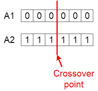
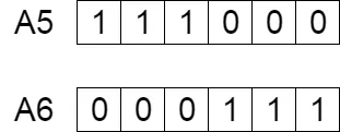
Crossover is the most significant phase in a genetic algorithm. For each pair of parents to be mated, a crossover point is chosen at random from within the genes.
For example, consider the crossover point to be 3 as shown below.
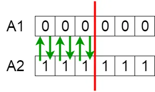
Offspring are created by exchanging the genes of parents among themselves until the crossover point is reached.
The new offspring are added to the population.
Mutation
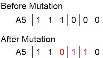
In certain new offspring formed, some of their genes can be subjected to a mutation with a low random probability. This implies that some of the bits in the bit string can be flipped.
Advantages of GAs
GAs have various advantages which have made them immensely popular. These include −
-
Does not require any derivative information (which may not be available for many real-world problems).
-
Is faster and more efficient as compared to the traditional methods.
-
Has very good parallel capabilities.
-
Optimizes both continuous and discrete functions and also multi-objective problems.
-
Provides a list of “good” solutions and not just a single solution.
-
Always gets an answer to the problem, which gets better over the time.
-
Useful when the search space is very large and there are a large number of parameters involved.
Limitations of GAs
Like any technique, GAs also suffer from a few limitations. These include −
-
GAs are not suited for all problems, especially problems which are simple and for which derivative information is available.
-
Fitness value is calculated repeatedly which might be computationally expensive for some problems.
The syntax that used in creating the genetic algorithm in MATLAB is as follows the different results and different case studies. Following is the syntax used in GA.
1. x=ga(fun,nvars) finds a local unconstrained minimum, x, to the objective function, fun. nvars is the dimension (number of design variables) of fun. where, fun- objective function and nvars-number of variables.
2. x=ga(fun,nvars,A,b,Aeq,beq,lb,ub) defines a set of lower and upper bounds on the design variables, x, so that a solution is found in the range lb≤x≤ub. (Set Aeq=[] and beq=[] if no linear equalities exist.)
3. x=ga(fun,nvars,A,b,[],[],lb,ub,nonlcon,lntCon) or x=ga(fun,nvars,A,b,[],[],lb,ub,nonlcon,lntCon,options) requires that the variables listed in lntCon take integer values.
Where, A and b are A=[] and b=[] if no linear inequalities.
lb and ub are lower bound and upper bound. Lower bounds, and upper bound specified as areal vector or array of doubles.
nonlcon is afunction that accepts a vector or array.
lntcon-integer variable vectors of positive integers.
options- Optimization options, specified as the outputnof optimoptions or a structure it helps in constraint tolerance by increasing the population size.
GOVERNING EQUATION:
To generate a stalagmite following functions are used,
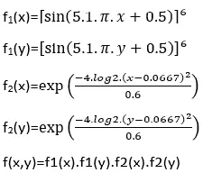
Maximizing f(x,y) s the same as minimizing -f(x,y)
FUNCTION CODE EXPLANATION:
Now using these values the stalagmite function is calculated. Function for the stalagmite is entered separately as a function code using the equations as mentioned above.
Now this function takes the 'input' values as the input for the function and the returns the values of 'f'.
Take the input values from the function x and y variables is stalagmite.
FUNCTION CODE:
MAIN CODE:
STUDY 1
To create the x and y variables by using the linspace command make the row wise vector.
Mesh the x and y variable by the meshgrid ( 2D array).
To evaluate the equation of stalagmite function in fir loop to give the input values to the function.
The tic works with the toc function to measure elapsed time. The tic function records the current time, and the toc function uses the recorded value to calculate the elapsed time.
x=ga(fun,nvars) finds a local unconstrained minimum, x, to the objective function, fun. nvars is the dimension (number of design variables) of fun. where, fun- objective function and nvars-number of variables.
CODE:
OUTPUT:
Basic stalagmite function and case study(1)
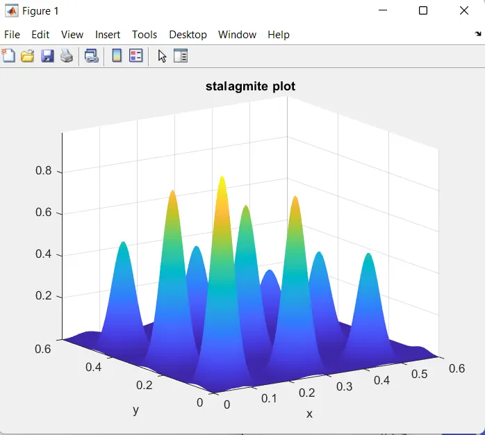
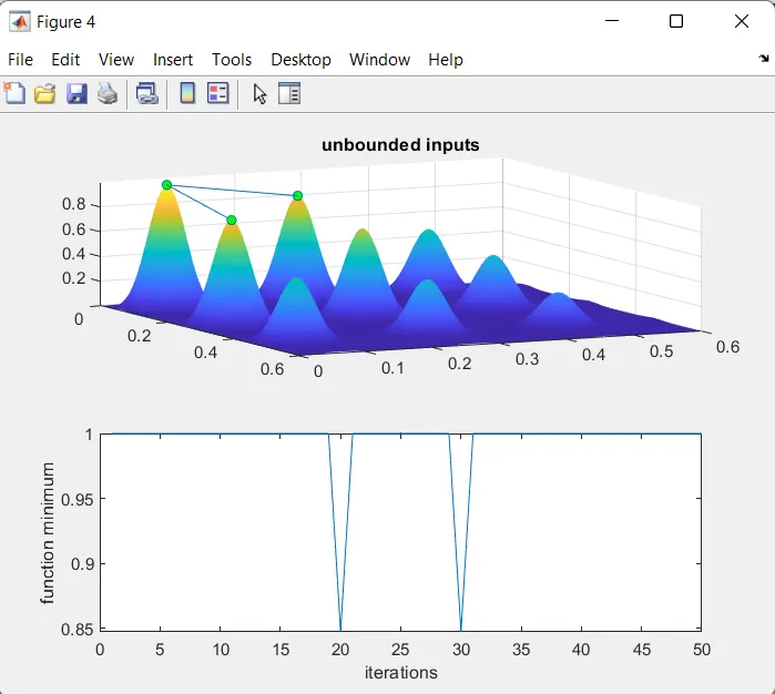
as we can see that there are more up-growing peaks, basically are my stalagmite structure. However, the function tends to give the negative value which gives the local minima's, so to make the function positive for getting the local and global maxima's. (upgrowing peaks). The highest peak is called global maxima and others are local maxima's.
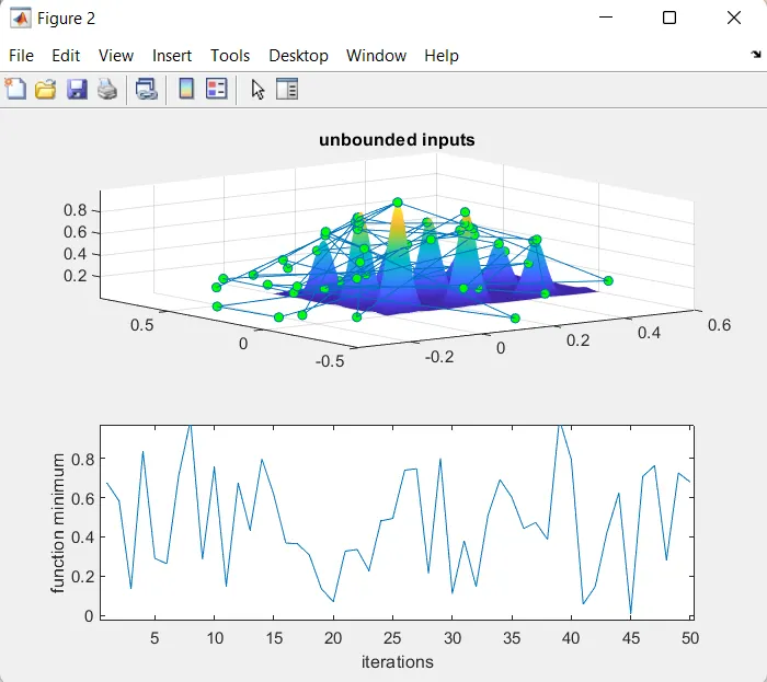
The solutions are not bounded so the GA will calculate all the possible maxima in'x' and 'y' coordinates.
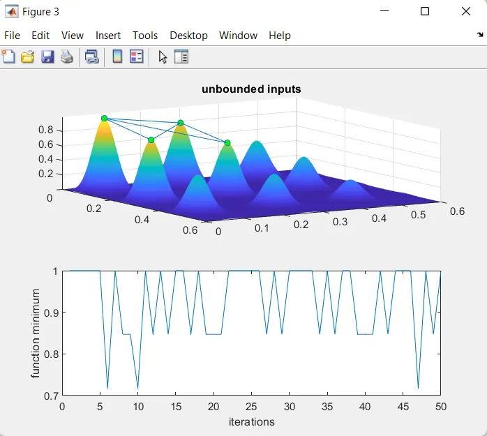
STUDY 2 CODE:
As the solution is dispersed in space we are limiting it to the global maxima simply we are converging the area for GA function for optimum values, on iterating the for loo[ for 50 times means we are evolving our solution to get better results for every generation to generation.
x=ga(fun,nvars,A,b,Aeq,beq,lb,ub) defines a set of lower and upper bounds on the design variables, x, so that a solution is found in the range lb≤x≤ub. (Set Aeq=[] and beq=[] if no linear equalities exist.)
CODE:
OUTPUT:
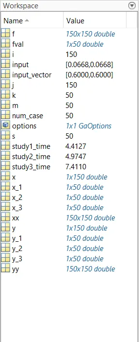
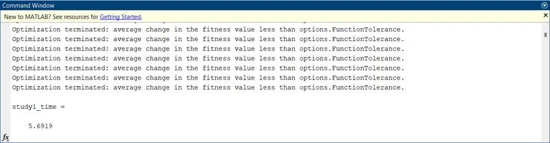
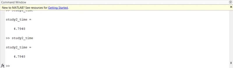
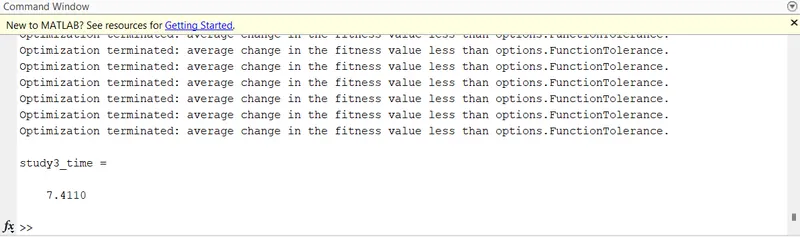
As we can see that the time taken in result two studies is
STUDY 3 CODE:
x=ga(fun,nvars,A,b,[],[],lb,ub,nonlcon,lntCon) or x=ga(fun,nvars,A,b,[],[],lb,ub,nonlcon,lntCon,options) requires that the variables listed in lntCon take integer values.
Where, A and b are A=[] and b=[] if no linear inequalities.
OUTPUT:
Which is approx 3 times greater than the case study one. As the population size is larger enough to carry out 50 iterations at the same time. however, we got our optimum maximized solution.
The time taken by the study 3 is
MATLAB FINAL CODE FOR ALL THREE STUDIES: