Project 2 - Rankine cycle Simulator
AIM:
To simulate a Ranking cycle using matlab.
Extracting steam and water properties from XSteam file.
Calculating all the state poits of the cycle based on User inputs.
Plotting the T vs S and H vs S plot for the given input.
INTRODUCTION:
The Rankine cycle closely describes the process by which steam engines commonly found in thermal power generation plants harness the thermal energy of a fuel or other heat source to generate electricity. Possible heat sources include combustion of fossil fuels such as cao,natural gas, or oil, renewable fuels like biomass or ethanol, nuclear fission, and concentrated solar power.
Required concepts:
Saturated liquid:
A liquid that is about to vaporize. At 1 atm and 20°C, water exists in the liquid phase (compressed liquid). At 1 atm pressure and 100°C, water exists as a liquid that is ready to vaporize (saturated liquid).
Saturated vapour:
vapor at the temperature of the boiling point corresponding to its pressure and so incapable of being compressed or cooled without condensing — compare equilibrium sense 1c.
Entropy:
The measure of a system's thermal energy per unit temperature that is unavailable for doing useful work. Because work is obtained from ordered molecular motion, the amount of entropy is also a measure of the molecular disorder, or randomness, of a system.
Enthalpy:
Enthalpy, a property of a thermodynamic system, is the sum of the system's internal energy and the product of its pressure and volume. It is a state function used in many measurements in chemical, biological, and physical systems at a constant pressure, which is conveniently provided by the large ambient atmosphere.
Processes of ranking cycle:
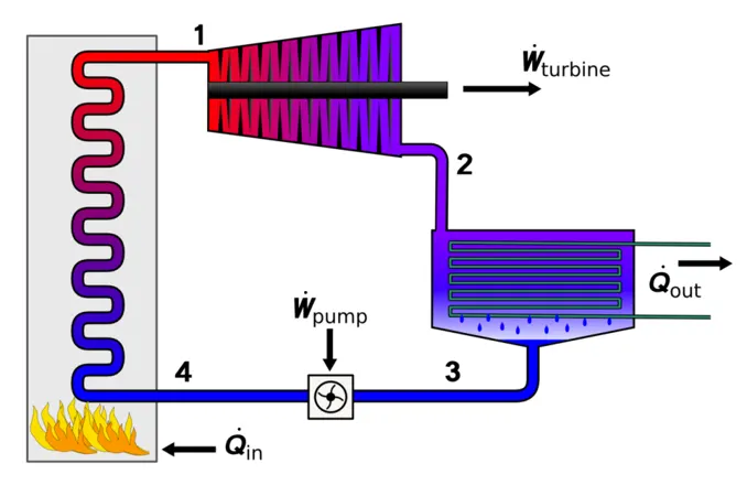
Heat energy is supplied to the system via a boiler where the working fluid (typically water) is converted to a high pressure gaseous state (steam) in order to turn a turbie. After passing over the turbine the fluid is allowed to condense back into a liquid state as waste heat energy is rejected before being returned to boiler, completing the cycle. Friction losses throughout the system are often neglected for the purpose of simplifying calculations as such losses are usually much less significant than thermodynamic losses, especially in larger systems.
Firstly, a pump is used in place o condenser to handle only liquid, not a mixture of liquid and vapour. Secondly, exhaust steam from the turbine is completely condensed in the condenser, see in the following diagram:
Processes and working:
There are four processes in the rankine cycle:
1. Process 1-2 : Isentropic Expansion in the turbine
2. Process 2-3 : Constant pressure Heat rejection in condenser
3. Process 3-4 : Isentropic compression in the pump
4. Process 4-1: Constant pressure heat addition in the boiler
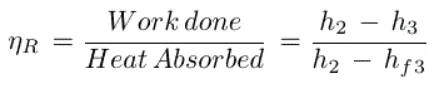
Rankine cycle efficiency ηR :
Back work ratio:
The fraction of the wprk produced by the turbine that is consumed by the compressor.
BW ratio=Wp/Wt
MAIN CODE:
clear all
close all
clc

% displaying processes of states
disp(' RANKING CYCLE ')
disp('1-2 is Constant pressure heat addition in the boiler');
disp('2-3 is Isentropic Expansion in the Turbine');
disp('3-4 is Constant presuure heat removal in the Condenser');
disp('4-1 is Isentropic compession in the pump');

% input for the rankine cycle data
p1=input('Value of pressure at turbine inlet, p1(in bar) =');
T1=input('Value of temperature at turbine inlet, T1(in degree.C) =');
p2=input('Value of pressure at condenser inlet inlet, p2(in bar) = ');

%At state 1
h1=XSteam('h_pT',p1,T1);                % Extracting Enthalpy at state pt 1
s1=XSteam('s_pT',p1,T1);                % Extracting Entropy at state pt 1

%At state 2
s2=s1;                                  % Isentropic Expansion
sf2=XSteam('sL_p',p2);                  % Saturated Liquid Entropy
sg2=XSteam('sV_p',p2);                  % Saturated vapour Entropy
x2=(s2-sf2)/(sg2-sf2);
hf2=XSteam('hL_p',p2);                  % Saturated vapour enthalpy
hg2=XSteam('hV_p',p2);                  % Saturated liquid enthalpy
h2=hf2+(x2*(hg2-hf2));

% At state 3
p3=p2;                                  % Constant pressure heat rejection in Condenser
s3=XSteam('sL_p',p3);                   % Saturated liquid entropy
h3=XSteam('hL_p',p3);                   % Saturated vapour entropy

% At state 4
s4=s3;                                  % Constant pressure heat addition in the boiler
p4=p1;

% work done by turbine
Wt=h1-h2;

%Work done to run pump
v3=XSteam('vL_p',p3);                   % Saturated liquid volume
Wp=v3*(p4-p3)*100;
h4=h3+Wp;

%Net work
Wnet=Wt-Wp;

%Heat into the system
Qin=h1-h4;

%Heat out of the system
Qout=h2-h3;

%Thermal efficiency
thermal_eff=(Wnet/Qin)*100;

%Specific steam consumption
%SSC=mass flow rate/power
SSC=(3600/Wnet);

% Back work ratio
BW=(Wp/Wt);

% Calculation of Temperature at the state points
T3=XSteam('Tsat_p',p3);                  % Saturation temperature
T2=T3;
Cp4=XSteam('Cp_ps',p4,s4);               % Specific isobaric heat capacity as a function of pressure and entropy.
Cv4=XSteam('Cv_ps',p4,s4);               % Specific isochoric heat capacity as a function of pressure and entropy.
k=Cp4/Cv4;
T4=T3/((p3/p4)^((k-1)/k));

% Calculating Temperature, Entropy and Enthalpy at the vapour and liquid line for plotting
T6=XSteam('Tsat_p',p1);                  % Saturation temperature
s5=XSteam('sL_p',p1);                    % Saturated liquid entropy
s6=XSteam('sV_p',p1);                    % Saturated vapour entropy
h5=XSteam('hL_p',p1);                    % Saturated liquid enthalpy
h6=XSteam('hV_p',p1);                    % Saturated vapour enthalpy
T5=T6;

%Plotting the sturation curve
T=linspace(1,375,1000);
for i=1:length(T)
    sf(i)=XSteam('sL_T',T(i));
    sg(i)=XSteam('sV_T',T(i));
    hf(i)=XSteam('hL_T',T(i));
    hg(i)=XSteam('hV_T',T(i));
end

cd("C:\Users\ramak\Pictures\Saved Pictures")

% plotting T-s diagram
figure(1)
hold on
plot(sf,T,'r','linewidth',1)
plot(sg,T,'r','linewidth',1)
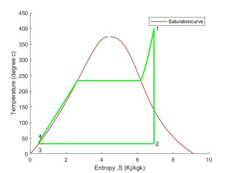
plot([s1 s2],[T1 T2],'g','linewidth',2)
plot([s2 s3],[T2 T3],'g','linewidth',2)
plot([s3 s4],[T3 T4],'g','linewidth',2)
plot([s4 s5],[T4 T5],'g','linewidth',2)
plot([s5 s6],[T5 T6],'g','linewidth',2)
sc1=linspace(s6,s1,1000);
for l=1:length(sc1)
    Tc1(l)=XSteam('T_ps',p1,sc1(l));
end
plot(sc1,Tc1,'g','LineWidth',2)
text(s1+0.1,T1,'1')
text(s2+0.1,T2,'2')
text(s3,T3-20,'3')
text(s4,T4+20,'4')
xlabel('Entropy ,S (Kj/kgk)')
ylabel('Temperature (degree c)')
legend('Saturationcurve')
saveas(figure(1),'T-S diagram.jpg')

% plotting h-s diagram
figure(2)
hold on
plot(sf,hf,'k','linewidth',1)
plot(sg,hg,'k','linewidth',1)
plot([s1 s2],[h1 h2],'g','linewidth',2)
plot([s2 s3],[h2 h3],'g','linewidth',2)
plot([s3 s4],[h3 h4],'g','LineWidth',2)
hc=linspace(h4,h5,100);
for r=1:length(hc)
    sch(r)=XSteam('s_ph',p1,hc(r));
end
plot(sch,hc,'g','linewidth',2)
plot([s5 s6],[h5 h6],'g','LineWidth',2)
for m=1:length(sc1)
    hc1(m)=XSteam('h_ps',p1,sc1(m));
end
plot(sc1,hc1,'g','linewidth',2)
text(s1+0.1,h1,'1')
text(s2+0.1,h2,'2')
text(s3,h3-100,'3')
text(s4,h4+200,'4')
title('Enthalpy vs Entropy plot')
xlabel('Entropy , S (KJ/kgk)')
ylabel("Enthalpy , H (KJ/kg)")
legend('Saturation curve','location','northwest')
saveas(figure(2),'H-S diagram.jpg')

% Displaying the result in the command window:
disp('result');
p1=p1;
T1=T1;
p2=p2;
disp('At stage point 1');
n1=sprintf('P1 is %.3f bar',p1);
disp(n1);
n2=sprintf('T1 is %d C',T1);
disp(n2);
n3=sprintf('h1 is %.3f KJ/kg',h1);
disp(n3);
n4=sprintf('s1 is %.3f KJ/kgk',s1);
disp(n4);
disp('At stage point 2');
n11=sprintf('P2 is %.3f bar',p2);
disp(n11);
n21=sprintf('T2 is %.3f C',T2);
disp(n21);
n31=sprintf('h2 is %.3f KJ/kg',h2);
disp(n31);
n41=sprintf('s2 is %.3f KJ/kgk',s2);
disp(n41);
disp('At stage point 3');
n12=sprintf('P3 is %.3f bar',p3);
disp(n12);
n22=sprintf('T3 is %.3f C',T3);
disp(n22);
n32=sprintf('h3 is %.3f KJ/kg',h3);
disp(n32);
n42=sprintf('s3 is %.3f KJ/kgk',s3);
disp(n42);
disp('At stage point 4');
n13=sprintf('P4 is %.3f bar',p4);
disp(n13);
n23=sprintf('T4 is %.3f C',T4);
disp(n23);
n33=sprintf('h4 is %.3f KJ/kgk',h4);
disp(n33);
n43=sprintf('s4 is %.3f KJ/kgk',s4);
disp(n43);
n14=sprintf('Wt is %.3f KJ/kg',Wt);
disp(n14);
n15=sprintf('Wp is %.3f KJ/kg',Wp);
disp(n15);
n16=sprintf('Wnet is %.3f KJ/kg',Wnet);
disp(n16);
n17=sprintf('Thermal_efficiency is %.2f percent',thermal_eff);
disp(n17);
n18=sprintf('SSC is %.2f kg/kWh',SSC);
disp(n18);
n19=sprintf('Back work ratio is %.3f',BW);
disp(n19);
CODE EXPLANATION:
- Displaying process of state such as Constant pressure heat addition in the boiler, Isentropic Expansion in the Turbine, Constant presuure heat removal in the Condenser, Isentropic compession in the pump.
- XSteam data is used to extract steam and water properties of entalpy, entropy at specific pressure and temperatures for saturated liquid, saturated vapour conditions etc.
- The program requires the input of pressure (in bar) at state point 1 (turbine inlet), Temperature at same point (degree celcius) and pressure at condenser inlet (point 2).
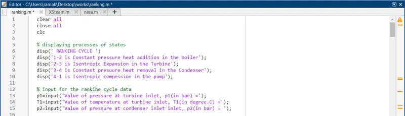
- With the help of these inlets & from XSteam data, the program calculates all the state points of the Rankine cycle.
- The XSteam data works as, h1=XSteam('h_pT',p1,T1) it returns the enthalpy of water at given pressure and temperature in bar and degC respectively.
- As we extract the data, we use thermodynamic relation to further find state points and extract their data from XSteam which are mentioned after studying the Rankine cycle.
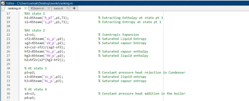
- Sf and sg, hf and hg, where f and g stands for saturated liquid and saturated vapour respectively are calculayed after studying the plots of Rankine cycles and extracting data from XSteam file.
- The net work, work done by turbine, work done to run the pump, Heat in and heat out are calculated using standard thermodynamic relation.
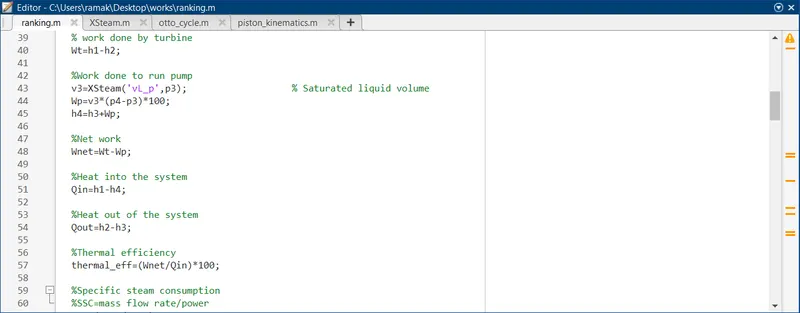
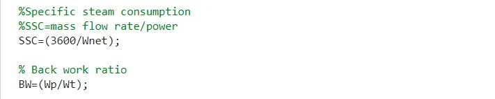
- Efficiency and Specific steam cinsumption (S.S.C) of the Rankine cycle is calculated from thermodynamic relations and mentioning them in program using relations.
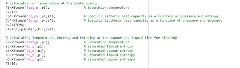
- T,s and h are extracted at vapour and liquid line for plotting purpose, after 4th point for the variation you observe in the plot.
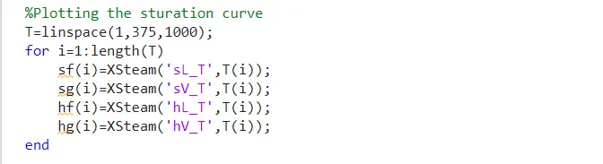
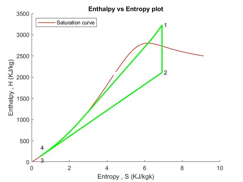
- Saturation curves is plotted in red for saturated liquid and saturated gas in T-S and H-S it is black.
- Plot of T vs S and h vs s is created from all the points obtained from the program using the plot command and mentioning all the labels, linewidth, color and title.
- The plot changes as the user input changes for the above mentioned inputs.
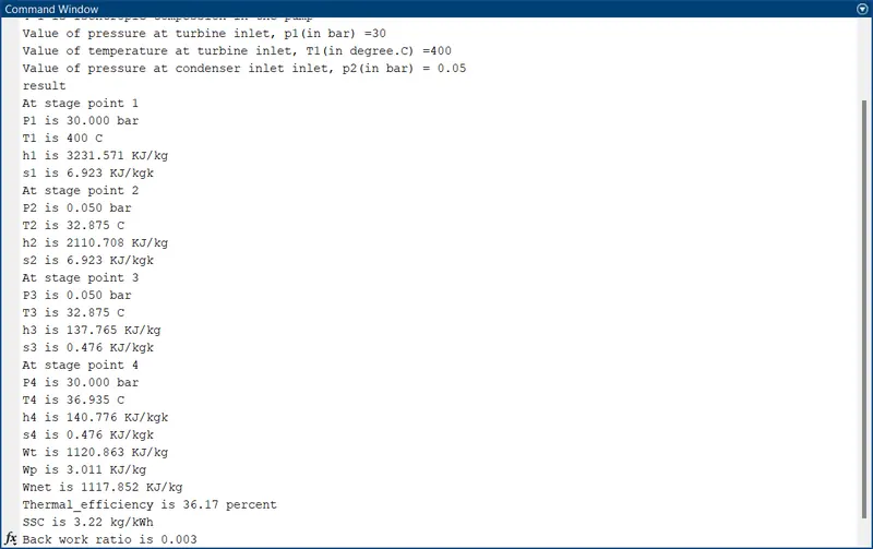
- Results are displayed in the command window by using sprint command.
ERROR:
Error occurs on the coding time that error is "Unrecognized function or variable 'linespace'.".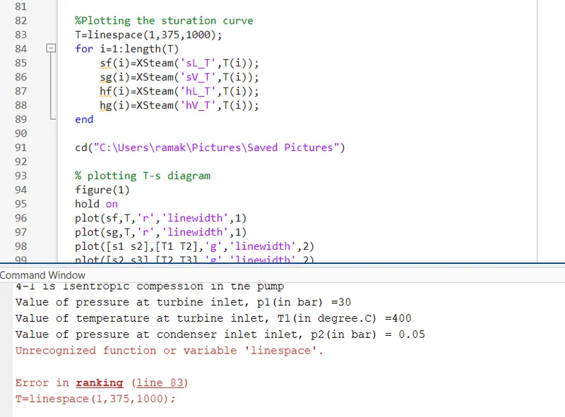
And rectifying the error by the correction of function (linespace = linspace) on the line number 83.
PLOTS AND RESULTS:
The plots of the Temperature and Entropy with labels and legends.
The plots of the Enthalpy and Entropy with the labels and legends.
The results of the variables and outputs of the stage wise outputs on the command windows.
REFERENCES:
https://en.wikipedia.org/wiki/Rankine_cycle
https://www.qrg.northwestern.edu/thermo/design-library/regen/regen.html