Week 4.1 - Genetic Algorithm

Aim: To find the global maxima of the respected stalagmite function by writing the code in Matlab programming.

Theory:

Here, our main objective is to find the best-optimized solution for our issue or program through an approach of Genetic algorithm which is to be applied to the stalagmite structure.

In this case, the GA(genetic algorithm)can only find the global or local minimum value. But, by using some simple inverse techniques, we are going to get the accurate global maximum.

GENETIC ALGORITHM (THE CONCEPT)

Genetic algorithm is mainly used to produce high-graded solutions to optimization problems by the use of the operators such as selection, crossover, and mutation.

At each procedure, the genetic algorithm selects the individuals from the current population into the category of parents and uses them to produce children for the next generation. Over the successive generations of selection, an optimized solution can be created or evolved.

so, the genetic algorithm contributes to finding the global minima for highly non-linear, non-differentiable, and stochastic( which cannot be predicted precisely) problems.

Primarily, Selection selects the individuals called parents, that contribute to the population for the further generation. It depends on the individual scoring.

for ex; from a large set of solutions, the two highest valued solutions are picked as parents for the crossover process.

Then, crossover combines two parents to form the solutions for next-generation and mutation applies random changes to individual parents to form children.

Anyways it differs from a classical algorithm(which generates only a single point at each iteration, and their sequence of points gets the main optimal solution).

whereas, The GA generates a population of points at each iteration, and the best point in the population approaches an optimal solution.

Here is the flowchart of genetic algorithm which demonstrates the stepwise flow of the process of GA,

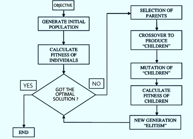
figure 1: represents the flowchart of the genetic algorithm

(this image is a replica of the flow chart of the genetic algorithm which is edited or made using Piscart application)

Syntax of GA(genetic algorithm) with examples ;

ga = (@(f), no. of variables)

Here, the ga defines the genetic algorithm, and the main syntax starts off by calling the function by using (@ (f)) and after calling the function, we should give the no of variables obtained by that respective function.

for ex: ga = (@stalagmite, 2)

here, we are calling the function called stalagmite, and the no of variables in that function's equations are mentioned after calling the function. here if only (x and Y) are the no of variables in that function, then it will be represented by 2. if it includes x, y, and z then it will be mentioned by 3, etc.

if there are any linear equalities or integer constraints mentioned in the equations of that function, then there are also represented in the function.

ga = (@stalagmite,2,[],[],[],[],[0:0],[0.6,0.6],[],[],options)

Here, the linear equalities are mentioned after the no. of variables and integer constraints should be mentioned after the boundaries values. They should be set to 4 linear equalities by default and two integer constraints. They should be mentioned if they are present otherwise they will have remained as Null vectors.

>> OPTIMIZING THE STALAGMITE FUNCTION AND FINDING THE GLOBAL MAXIMA ;

So here, we are imagining or framing a situation for ourselves and assuming it in a stalagmite function for obtaining its optimal solution.

TASK;

(a picture representing the location where global maxima to be found)

Here, among the group of tallest mountains, an organization wants to know the tallest point of this landscape to built a view point for tourists. So, we need to find the maximum peak point of this location. For that, we need to find the optimized solution of the Global Maxima by using the stalagmite function and using the genetic algorithm method in an inverse way to get the maxima.

THE EQUATIONS OR FORMULAS;

`f1,x = [sin(5.1*pi*x+0.5)]^6`

`f1,y = [sin(5.1*pi*y+0.5)]^6`

`f2,x = exp[-4ln(2)*((x-0.0667)^2/0.64)]`

`f2,y = exp[-4ln(2)*((y-0.0667)^2/0.64)]`

Here, we need to get this equations into the stalagmite function by converting them to a coded form in Matlab programming.

THE STALAGMITE FUNCTION;

function[f] = stalagmite(input_vector)
fx =(sin(5.1*pi*input_vector(1)+0.5))^6;
fy =(sin(5.1*pi*input_vector(2)+0.5))^6;

fxx = exp(-4*log(2)*((input_vector(1)-0.667)^2/0.64));
fyy = exp(-4*log(2)*((input_vector(2)-0.667)^2/0.64));

f =-(fx*fy*fxx*fyy);
end

This is the respected stalagmite function which is neede to be called by GA.

THE MAIN CODE PERFORMING GENETIC ALGORITHM;

clear all
close all
clc

%defining our search space
x = linspace(0,0.6,150);
y = linspace(0,0.6,150);

%creating a 2dimensional mesh

[xx, yy] = meshgrid(x, y);

%evaluating the stalagmite function
for i = 1:length(xx)
    for j = 1:length(yy)
        input_vector(1) = xx(i,j);
        input_vector(2) = yy(i,j);
        f(i,j) = stalagmite(input_vector);
    end
end
f = -f
surfc(xx,yy,f)
xlabel('x value')
ylabel('y value')

shading interp

[inputs, fval] = ga(@stalagmite, 2)

EXPLAINATION OF THE CODE;

Starting with the basics like clear all, close all, and clc

We have created our search space for the optimized solution with 1D arrays (x and y) and converted them into a 2D array by using the meshgrid() command.

For each value of x and y, we are creating an array called input_vector(row vector which has 2 columns).

And now we have the function called stalagmite, which takes in the input_vector and calculates the 'f'.

That 2 for loops will generate the data for the plot of stalagmite.

surfc is used to visualise the function (xx, yy, f)'

shading interp is used to remove the gridlines and represents the smooth gradient way.

Finally, we are generating the GA (an inbuilt solver).

@stalagmite represents the function that is to be minimized and mentions the number of variables inside the function (that is 2).

OUTPUT AND PLOT AFTER EXECUTING THE ABOVE PROGRAM;

inputs =

    0.8453    0.6240


fval =

   -0.3884

.

PLOT;

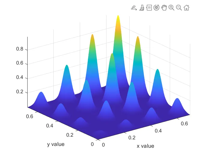
we are getting the minimum input values which are nearer to 0.

because GENETIC ALGORITHM GENERATES THE GLOBAL MINIMA and LOCAL MINIMA. But, we need the GLOBAL MAXIMA.

For that, we need to modify the program along with the stalagmite function for getting the peak value of this funtion.

FOR GETTING THE GLOBAL MAXIMA VALUE;

we need to inverse the function ( f = -f)

Studying the statistical behaviour of the genetic algorithm code; (STUDY-1)

close all
clc

x = linspace(0,0.7,150);
y = linspace(0,0.7,150);
num_cases = 50;

[xx, yy] = meshgrid(x, y);

% f = stalagmite(x,y);

for i = 1:length(xx)
    for j = 1:length(yy)
        input_vector(1) = xx(i,j);
        input_vector(2) = yy(i,j);
        f(i,j) = stalagmite(input_vector);
    end
end
tic
%study 1 - the statistical behaviour
for i = 1:num_cases
    [inputs, fopt(i)] = ga(@stalagmite,2);
    xopt(i) = inputs(1);
    yopt(i) = inputs(2);
   
end
study1_time = toc
f = -f
fopt = -fopt
figure(1)
subplot(2,1,1)
hold on
surfc(x,y,f)
shading interp
plot3(xopt,yopt,fopt,'marker','o','markersize',5,'markerfacecolor','r')
title('unbounded inputs')
subplot(2,1,2)
plot(fopt)
xlabel('Iterations')
ylabel('Function minimum')

EXPLANATION OF STUDY-1;

Here, we studied the statistical behaviour of the function with the help of two plots in a figure.

subplot command is used to create the desired number of plots in a single figure which can be used for detailed comparison.

we have used the hold on command to set the two plots working at same time,instead of getting the recent one.

we have plotted the fopt( which is a combined point of xopt and yopt) with desired marker style and markersize along with its color.

Then, x and y axis is labelled.

OUTPUT AND PLOT OF STUDY 1(the statistical behaviour);

The output will be the f which is 150x150 double (x and y) values and values are will be mentioned through columns 1-150. And the study time is approximately about 3.443 seconds.

PLOT;

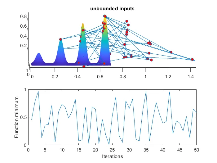
Here, we can see the various number of inputs that will get closure to the optimal solution by iterations.

But here, due to no boundaries set,GA did not recognize that the values can go beyond 0 and above 0.7. So, we need to set the boundaries of min and max.

Then the optimal solutions will be filtered better than this statistical unbounded inputs behavior. we need study 2 for the next step filtration.

STUDY-2 (INCLUDE THE UPPER AND LOWER BOUNDS FOR BETTER OPTIMAL SOLUTION);

CODE:

%study 2 -the statistical behaviour (upper and lower bounds)
tic
for i = 1:num_cases
    [inputs, fopt(i)] = ga(@stalagmite,2,[],[],[],[],[0;0],[0.7;0.7]);
    xopt(i) = inputs(1);
    yopt(i) = inputs(2);
   
end
study2_time = toc;
fopt = -fopt;
f = -f
figure(2)
subplot(2,1,1)
hold on
surfc(x,y,-f)
shading interp
plot3(xopt,yopt,fopt,'marker','o','markersize',5,'markerfacecolor','r')
title('bounded inputs')
subplot(2,1,2)
plot(fopt)
xlabel('Iterations')
ylabel('Function minimum')

It is similar to study-1. But Here, we are setting the upper and lower bounds for filtration of optimized solution. we are also including the null vectors [], which are to be filled if there are linear equalities inside the objective to be done.

OUTPUT AND PLOT OF STUDY-2;

output will be of the f values(150x150) double, and dispalyed as columns through 1-150. and the study time is approximately upto 3.8767 seconds

PLOT;

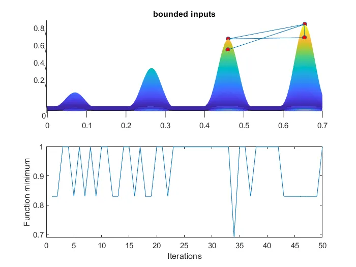
If we observe clearly, we have got the best optimal solutions from the various solutions for this study-2. There are nearly 3-4 optimal solutions representing the global maxima or the peak point. we are close to the exact optimized solution now.

As we now GA starts with the random sampling, by default the GA will take the 50 num cases.

We will get the best accurate optimal solution if we increase the population.

170,190,200 can give the best single optimized global maxima. So, here I am going to take the population size as 170.

STUDY-3 (INCREASING THE POPULATION SIZE FOR ACCURATE GLOBAL MAXIMA);

CODE:

%study 3 - increasing the GA population

options = optimoptions('ga');
options = optimoptions(options,'populationsize',170);

tic
for i = 1:num_cases
    [inputs, fopt(i)] = ga(@stalagmite,2,[],[],[],[],[0;0],[0.7;0.7],[],[],options);
    xopt(i) = inputs(1);
    yopt(i) = inputs(2);
   
end
study3_time = toc;
fopt = -fopt;
f = -f
figure(3)
subplot(2,1,1)
hold on
surfc(x,y,f)
shading interp
plot3(xopt,yopt,fopt,'marker','o','markersize',5,'markerfacecolor','r')
title('bounded inputs with modified population size')
subplot(2,1,2)
plot(fopt)
xlabel('Iterations')
ylabel('Function minimum')

Here, we have mentioned the population size as 170, which was set to be 50 by default in GA. And, the integer constraints can be mentioned if there are any in the objective.

As now they are kept as Null vectors only.

OUTPUT AND PLOT OF STUDY-3;

oOutput will be f (150x150) values of (xx and yy) and mentioned through columns 1-150 in the command window. The study time is approximately about 8.373 seconds

due to increase in population size, the execution time is taken longer than in the previous studies.

PLOT;

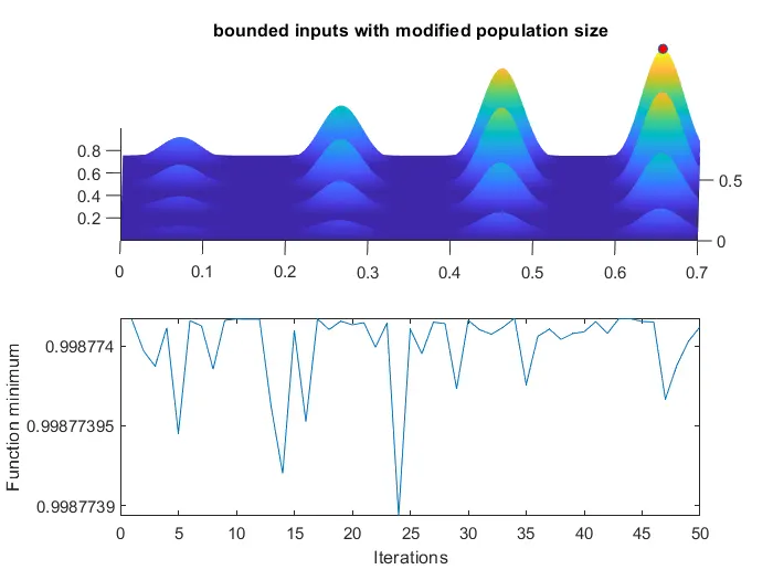
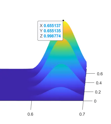
So, Finally by increasing the population size, we got the accurate (optimized solution) GLOBAL MAXIMA for our stalagmite function. (at X = 0.655137, Y = 0.665135)

(According to the TASK imagination, we can build the view point at that accurate point of the tallest mountain.)

ERRORS OCCURED IN MY CODING;

1) I have forgotten to inverse the study 3 plot, so I got the plot presentation downwards which is reflecting the global minima.

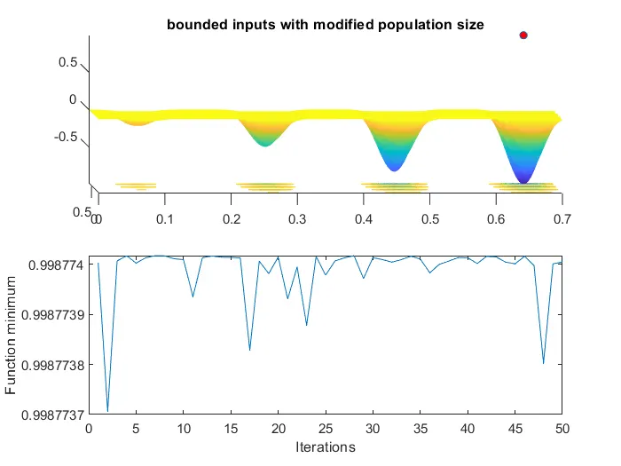
figure representing the non-inverse direction of the plot which is not suitable for global maxima

After inverting it with a single statement (f = -f) issue got resolved.

2) I have not mentioned the null vectors of linear equalities, so the program is not executed, mentioning this;

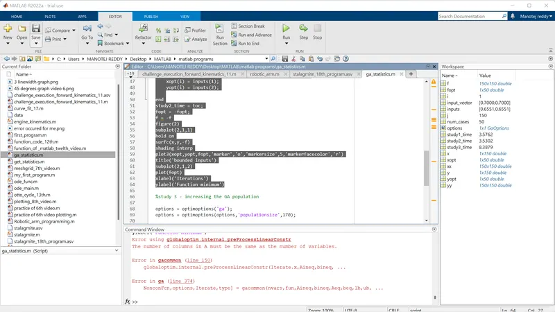
After mentioning the null vectors by researching about the syntax of the genetic algorithm(ga), the issue was resolved and the plot is executed.

Conclusion;

Finally, we got the global maxima of the stalagmite function,

By step by step procedure of-

Setting the upper and lower boundaries

Increasing the population and slowly getting towards the accurate filtered optimal solution.

references;

Mathworks official page of information'

Holland, J. H. (1992). Genetic algorithms. Scientific American, 267(1), 66–73.

Geeks for Geeks article about Genetic algorithms.

https://www.geeksforgeeks.org/genetic-algorithms/

THANK YOU