Project 2 - Rankine cycle Simulator
Rankine Cycle Simulator
Aim: To Create the Rankine cycle simulator from the given input and read the data from the standard thermodynamics library of the steam table.
Objective: Our objective is to construct the Rankine cycle simulator using MATLAB Programming, and to calculate the state points using the function Xsteam.
To Plot T-S and H-S curves for a given input of the Rankine cycle and to display the output in the Command window for each state point in the cycle.
Theory:
The Rankine cycle is a vapour powered cycle. This cycle is similar to the Carnot cycle. But in rankine we use Pump for handling the liquid or water, where as compressor is used in carnot for the process. Rankine is different from the gas-powered cycle in which the working fluid is gas in that process. In vapour powered cycle. the working fluid is steam because of its many desirable characteristics such as low cost of production, and greater enthalpy of vapourization.
1) Isentropic expansion
2) Constant pressure heat rejection (Towards condenser)
3)Isentropic compression
4)Constant pressure heat addition (Towards boiler)
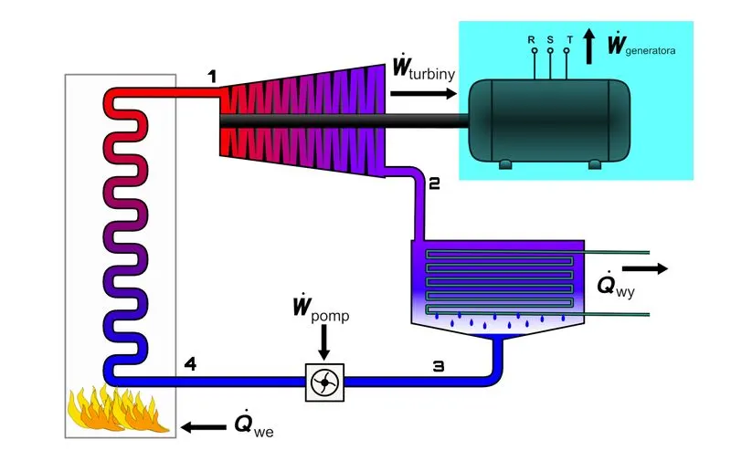
Figure representing the basic functioning of a Rankine cycle (modified by using PicsArt app)
Here we can see that the heat energy is supplied to the system via a boiler(state point 4), where the working fluid (mostly water) is converted to a high-pressure gaseous state which forces the turbine to get its momentum of rotation.(Hence the work begins now the electric generation starts which is connected to a turbine moment axle). After passing through the turbine, the fluid is allowed to condense back into a liquid state as waste heat energy is rejected before being returned to the boiler. And after the fluid is returned to the boiler. the process repeats similarly. And hence some amount of energy is waste as there is no system that can use its 100% energy is vice versa. But the energy which is wasted in the process is negligible. These Thermodynamic losses are common in this type of heat generation and usage works.
(The blue bordered section in the diagram indicates the power converted from mechanical to electrical and managed by the generator with gears)
Detailing of the four working process ongoing:
process 1-2 (Isentropic Expansion): The dry saturated vapour expands through a turbine, generating power. This decreases the temperature and pressure of the vapour, and some condensation may occur.
`Wt = h1- h2`
process 2-3 (Constant pressure Heat Rejection): Here, the vapour-liquid mixture leaving the turbine is condensed at low pressure, usually in a surface condenser using the low temperature water or fluid. mainly in well constructed condensers, the pressure of the vapour is below the atmospheric pressure only.
`Q1= h2 - h3`
Process 3-4 ( Isentropic Compression): Here, the pressure of the condensate is raised to the feed pump. Becuase the low specific volume of liquids, the pump work is relatively small and often neglected in thermodynamic calculations.
`Wp = h4 - h3`
Process 4-1 ( Constant pressure Heat Addition) : At this stage, the very high pressured liquid now enters the boiler from the feed pump and heated to the saturated temperature. Furtherly due to increase in heat energy, evaporation of the liquid begins until its completely converted into a saturated steam or super heated steam.
`Q2 = h1 - h4`
These are the working process at each stage of our Rankine cycle.
The thermal efficiency of a Rankine cycle can be obtained by,
Wnet = Wt - Wp
`eta_(thermal) = (Wnet/qi)*100
where
Wt = H1-H2
Wp = H4-H3
Qi = H1-H4
Qout = H2-H3
specific steam consumption
S.S.C = 3600/Wnet
Back work ratio can be derived by;
`.W.R = (H1-H4)/(H2-H3)`
Main Code:
clear all
close all
clc

%process information
fprintf('Rankine Cycle Simulator n')
fprintf('process 1-2: Isentropic Expansion n')
fprintf('process 2-3: Isobaric Heat Rejection n')
fprintf('process 3-4: Isentropic comprerssion n')
fprintf('process 4-1: Isobaric heat addition process n')

%Intial Inputs
P1 = input('Enter the inlet pressure of Turbine:')
P2 = input('Enter the outlet pressure from Turbine:')
T1 = input('Enter the steam inlet Temperature:')

%state point 1
H1 = XSteam('h_pt',P1,T1); %Enthalpy
S1 = XSteam('s_pt',P1,T1); %Entropy
Hf1 = XSteam('hL_p',P1); %Enthalpy of saturated liquid
Hg1 = XSteam('hV_p',P1); %Enthalpy of saturated vapour
Ts1 = XSteam('Tsat_P',P1); %Saturation temperature
Sf1 = XSteam('sL_p',P1); %Entropy of saturated liquid
Sg1 = XSteam('sV_p',P1); %Entropy of saturated vapour

%state point 2
S2 = S1;
Sf2 = XSteam('sL_p',P2);
Sg2 = XSteam('sV_p',P2);
Hf2 = XSteam('hL_p',P2);
Hg2 = XSteam('hV_p',P2);
x = (S2-Sf2)/(Sg2-Sf2); %Dryness fraction
H2 = Hf2+x*(Hg2-Hf2);
T2 = XSteam('T_ph',P2,H2);

%state point 3
H3 = Hf2;
S3 = Sf2;
T3 = T2;
P3 = P2;

%State point 4
P4 = P1;
S4 = S3;
H4 = XSteam('h_ps',P4,S4);
T4 = XSteam('T_ps',P4,S4);

t = linspace(0,374,500);

%plot T-S Diagram
figure(1)
hold on
 for i=1:length(t)
     plot(XSteam('sL_T',t(i)),t(i),'.','color','b')
     plot(XSteam('sV_T',t(i)),t(i),'.','color','b')
 end

 %plot cycle
 plot([S1,S2],[T1 T2],'linewidth',2,'color','r')
 if x>1
     T3 = Ts2;
     plot([S2 Sg2 S3 S4],[T2 Ts2 T3 T4],'linewidth',2,'color','r')
T2 = Ts2;
 else
     plot([S2 S3 S4],[T2 T3 T4],'linewidth',2,'color','r');
 end

 l = linspace(T1,T2,1000)

 for i=1:length(l)
     plot(XSteam('s_pT',P1,l(i)),l(i),'.','color','r')
 end
 plot([Sf1 Sg1],[Ts1 Ts1],'linewidth',2,'color','r')
 xlabel('Entropy[KJ/Kg-K]')
 ylabel('Temperature[K]')
 title('T-S Diagram')


%Plot H-S diagram
figure(2)
hold on

%Plot Saturation Curve
for i= 1:length(t)
plot(XSteam('sL_T',t(i)),XSteam('hL_T',t(i)),'.','color','b')
plot(XSteam('sV_T',t(i)),XSteam('hV_T',t(i)),'.','color','b')
end

%Plot cycle
plot([S1 S2 S3 S4 S1],[H1 H2 H3 H4 H1],'linewidth',2,'color','r')
xlabel('Entropy[KJ/Kg-K]')
ylabel('Enthalpy[KJ/Kg]')
title('H-S diagram')

%calculation

%Turbine work
wt = H1-H2;

%pump work
wp = H4-H3;

%Heat Addistion
Qin = H1-H4;

%Heat Rejection
Qout = H2-H3;

%Net work
Wnet = wt-wp;

%Efficiency
Ntherm = (Wnet/Qin)*100

%Specific stem consumption
SSC = 3600/Wnet;

%Back power Ratio
BWR = wp/wt;

%Print Result
fprintf('nnResults\n')
fprintf('At state point 1:\n')
fprintf('P1 is : %.2f bar\n',P1)
fprintf('T1 is : %.2f Deg Celcius\n',T1)
fprintf('H1 is %.2f KJ/Kg\n',H1)
fprintf('S1 is %.2f KJ/Kg-K\n',S1)

fprintf('nAt state point 2:\n')
fprintf('P2 is : %.2f bar\n',P2)
fprintf('T2 is : %.2f Deg Celcius\n',T2)
fprintf('H2 is %.2f KJ/Kg\n',H2)
fprintf('S2 is %.2f KJ/Kg-K\n',S2)

fprintf('nAt state point 3:\n')
fprintf('P3 is : %.2f bar\n',P3)
fprintf('T3 is : %.2f Deg Celcius\n',T3)
fprintf('H3 is %.2f KJ/Kg\n',H3)
fprintf('S3 is %.2f KJ/Kg-K\n',S3)

fprintf('nAt state point 4:\n')
fprintf('P4 is : %.2f bar\n',P3)
fprintf('T4 is : %.2f Deg Celcius\n',T4)
fprintf('H4 is %.2f KJ/Kg\n',H4)
fprintf('S4 is %.2f KJ/Kg-K\n',S4)


fprintf('nWt is : %,2f KH/Kg/n',wt)
fprintf('Wp is : %.2f KJ/Kg\n',wp)
fprintf('Wnet is  : %.2f KJ/Kg\n',Wnet)
fprintf('Thermal Efficiency is : %.2f percent\n',Ntherm)
fprintf('S.S.C is : %.2f Kg/KWh\n',SSC)
fprintf('Back Work Ratio is %.3f \n',BWR)
Explanation of the code:
Here, the code begins with the usual lines clc,clear all and close all.
Xsteam data is used to extract steam and water properties of enthalpy, entropy at specific pressure and temperature for saturated liquid and saturated vapour conditions.
Then, using fprintf command, we have intiated the title as Rankine cycle simulator and then mentioned all the four state points from 1-4 as above.
After mentioning the process information,as a part of initial inputs, we have typed the P1, P2 and T1 which can be used for any values later on. This inputs have been inputed after running the program by mentioning the values in the command window.
Here by, we are inserting the state points information by calling the XSteam file and inserting the H, S, P, and T values for every state point, so after the execution of the code, these commands can be calculated at the statepoint locations. With the help of these inlets from XSteam data, the program calculates all the state points of the Rankine cycle.
XSteam data can be functioned as, h1 = XSteam('h_pT',p1, T1); Which returns the enthalpy of the fluid(water) at a given pressure and temperature in bar and degrees respectively.
Similarly, these extraction of the data from Xsteam data goes on in an ordered way.
Then after, we have mentioned the temperature in the form of an array to get the values of it to a certain limit. and after, we plot the cycle with required inputs and measurements regarding linewidth, color and marker. using legend command specifies the curve well. we have even mentioned the xlabel and ylabel details and titled the plot graph.
Turbine work, pump work, heat addition, and heat rejection, net work done, Thermal efficiency etc are initiated for their calculation.
Here, as we see the inputs like Sf and sg, hs and hg. This means f stands for saturated liquid and g stands for saturated vapor respectively.
Net work done, total work done by the turbine, work done to run the pump, Heat in, and Heat out are calculated using standard thermodynamic relations.
Efficiency and Specific steam consumption (s.s.c) of the Rankine cycle are calculated.
Now, T,s and h are extracted at vapor and liquid lines for plotting purposes.
The saturated curve is plotted in red for saturated liquid and saturated gas.
Plot os T vs S and H vs S is then created from all the points from the code.
Hence, the plot changes according to the uses inputs given by the user, as we input some commands at the initial using the fprintf command.
Hence the details of the total inputs for the state points will be displayed in the command window after we execute.
Commands used in the code:
clc, clear all, close all: Usual commands which will be used at the start of the code for clearing, closing and removing the typed content in command window.
Input: This command is used to get the values of input conditions the from user
Xsteam: custom function to get values from steam table.
if-else : We initiated this command to calculate the dryness fraction s2.
for : This loop is used to create the points to plot dry saturated liquid and vapor lines.
Plot: The plot command is used to create the graph based on the input.
Text: This command helps in inserting the needed text at certain points or locations
fprintf: This command is used to print the required lines in the command window.
Results of T-S and H-S diagram:
T-S diagram;
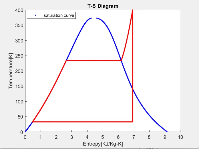
Here, the graph shows the Temperature vs Entropy. Here we can see the (saturation curve which is also represented by legend). Xlabel mentions the Entropy and Ylabel mentions the Enthalpy as shown.
H-S diagram;
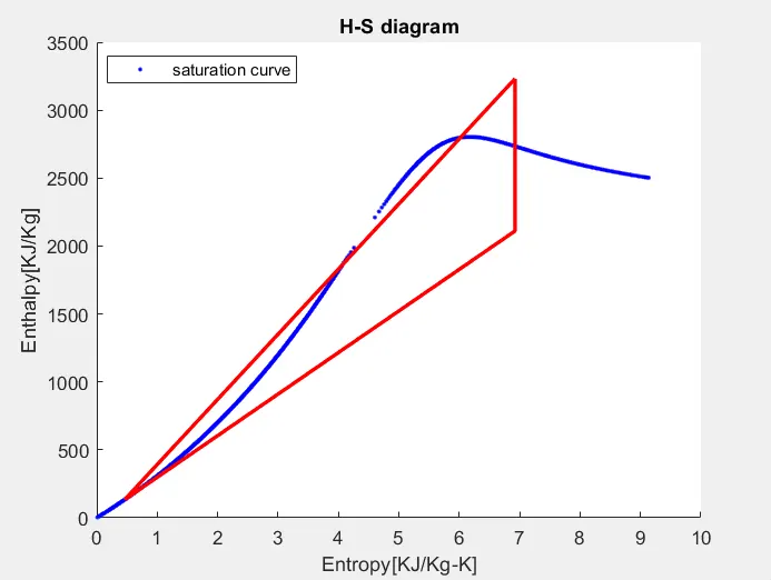
Graph mentioning about the Enthalpy vs Entropy and here the curve indicates the saturated curve. Xlabel mentions the Entropy and Ylabel mentions the Enthalpy as shown.
Detailings (outputs) in Command window:
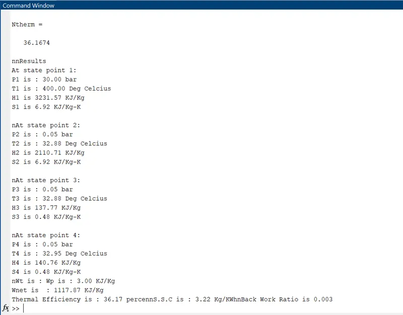
Here, we can see the state point detailings at each state which include Pressure(constant), Enthalpy, Entropy and Temperature calculations under each state over its cycle.
Thermal efficiency and Specific steam consumption (SSC) along with the BAck Work Ratio (BWR) are mentioned.
Workspace Information;
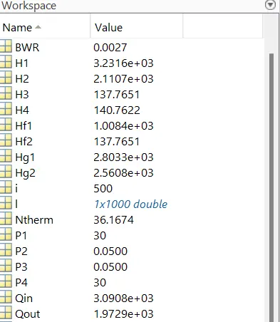
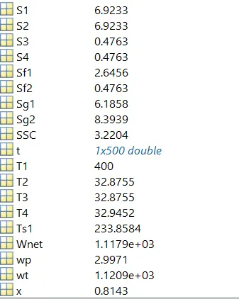
These are the enthalpy(H), Entropy(S), Temperature, Pressure, Heat in, and Heat out values along with thermal efficiency. We can see that t and L are in the form of arrays.
ERRORS FACED DURING CODE SECTION:
1. Since the code is intially inputed by the extraction of the data from a single data.file throughout (XSteam.m). I have used Xsteam instead of XSteam (used small 's' and got error as below,
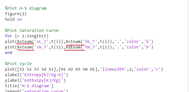
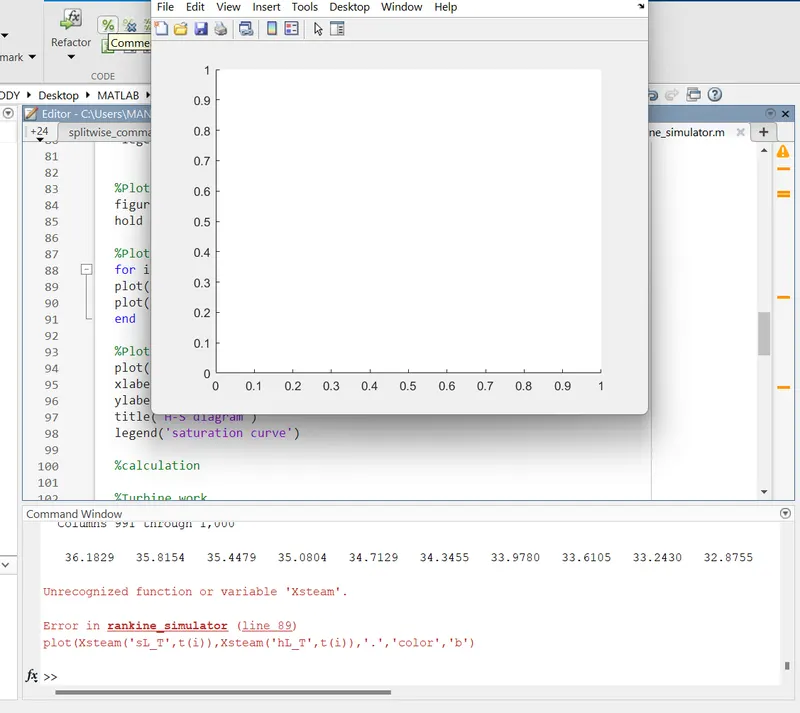
later by fixing the line 89 as indicated in the command window with the correct letter, the issue got resolved.
2. Secondly, I have used the newline command, but doesnt included the '\' key. Then got the values in the command window in a serial format as shown in the second figure.
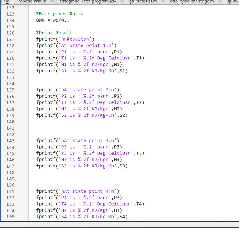

Then observed that is projection of results is in an abnormal way and inserted '\' at every line. Then got the result in an ordered way.
Conclusion: Hence, we have found the state points of the given Rankine cycle with the help of initial given values ( inlet and outlet pressure along with Temperature), and plotted the graphs of T-s and h-s along with finding the thermal efficiency of the Rankine cycle.
References: