Week 3 - Solving second order ODEs

Aim: To solve the ODE (second-order), which represents the equation od motion of a simple pendulum with damping.

Objective:

To write a code or program that solves the following ODE (of 2nd order), that represents the equation of motion of a simple pendulum with damping and also create an animation video from the output that obtains by solving this order equation.

`d^2theta/dt^2+b/m*d(theta)/dt+g/L*sintheta = 0`

Theory:

The motion of the pendulum represents the simple harmonic motion (SHM), which consists of a small bob along with the string holding it with damp. This whole moment is depended on Newtons second law of motion.Here the below daigram gives a brief idea about the pendulum and its motion.

Figure 1

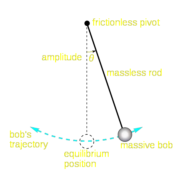
Represents the motion of a bob with SHM.

As shown, the bob with a certain mass which is damped by using a massless string is under simple harmonic motion, we need to derive this particular motion using the second order ODE

given in this respective assignment. That is,

`d^2theta/dt^2+b/m*d(theta)/dt+g/Lsin(theta)=0`

from the above equation,

b = damping coefficient

m = mass of the ball (kg)

g = gravity in m/s^2

L = length of the repective pendulum (m = meters)

The given is a form of 2nd order ODE equation, so we need to convert it into two first-order equations to solve the ODE.

`theta=theta1`

`d(theta1)/dt=theta2`

``d^2(theta)/dt^2=d(theta2)/dt`

Given dimensions;

L = 1 metre

m = 1kg

b = 0.05

g = 9.81 m/s^2 ( mostly a constant)

here are my assumed calculations,

Timespan = 0-17 sec

Intial displacement = 0

Intial velocity = 3 m/s at time, t = 0.

CODE FOR THE EQUATION;

 clear all
 close all
 clc

 b = 0.05;
 g = 9.81;
 l = 1;
 m = 0.1;

 %initial conditions
 theta_0 = [0;3];

 % time points
 t_span = linspace(0,20,500);

 % solve ODE
 [t, results] = ode45(@(t,theta)ode_func(t,theta,b,g,l,m),t_span, theta_0);

 plot(t,results(:,1)) 
 hold on 
 plot(t,results(:,2))
 ylabel('plot')
 xlabel('time')
 legend('displacement','velocity')

EXPLANATION;

Here, the code starts with the usual commands,

then we inputed the values given to the ODE into the program.

The intial conditions are represnted by 0 (Displacement) and 3 ( velocity at start).

Assumed t_span (duration) is 0-20 seconds with 500 values in between.

And to solve this ODE, we are using the ode45@ which is an inbuilt solver for this kind of problems. Then we mentioned t_span, theta along with the function calling ode_func.

Then plotting the results of time along with the x and y-axis for the mentioned time.

Then we have legend command for clear distinguistion

ODE FUNCTION TEMPLATE;

function [dtheta_dt] = ode_func(t,theta,b,g,l,m)

theta1 = theta(1)
theta2 = theta(2)
dtheta1_dt = theta2;
dtheta2_dt = -(b/m)*theta2 - (g/l)*sin(theta1);
dtheta_dt =  [dtheta1_dt; dtheta2_dt];
end

This is the respective function we built for directly inputting into the program for getting the input argument values within this.

We have defined theta1 and theta2 inside it.

We have also mentioned our splitted 2nd order equations which are two single order equations now.

This function gives the time and results for our ODE.

OUTPUT OF THE RESULTS AND ITS WORKSPACE;

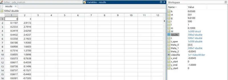
We can observe that the results is an array now. There are 500x2 rows and columns representing the motion of the pendulum for 17 seconds at each of the 500 values. We got this values by the calculation of t and t_span values.

GRAPH REPRESENTING THE MOTION FOR THE DURATION OF DISPLACEMENT AND VELOCITY;

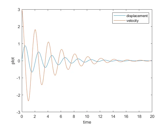
Here, the curve which travels from 0 is a displacement curve as it is starting from 0, and the other curve is a velocity curve of initial velocity 3m/s. Legend command is used for clear identification of both the curves.

PROGRAM FOR ANIMATING THE ABOVE EQUATION;

As we have learned how to animate the program or any function from the Forward kinematics solutions, here are animating the pendulum motion of that ODE.

CODE FOR ANIMATION;

 clear all
 close all
 clc

 b = 0.05;
 g = 9.81;
 l = 1;
 m = 0.1;

 %initial conditions
 theta_0 = [0;3];

 % time points
 t_span = linspace(0,20,500);

 % solve ODE
 [t, results] = ode45(@(t,theta)ode_func(t,theta,b,g,l,m),t_span, theta_0);

 plot(t,results(:,1)) 
 hold on 
 plot(t,results(:,2))
 ylabel('plot')
 xlabel('time')
 legend('displacement','velocity')

 %For loop for animating the simple pendulum.

 ct = 1;
 theta_1 = results(:,1);
 for i = 1:length(results(:,1))
    
   %intial conditions
   x_start = 0;
   y_start = 0;
   theta_2 = theta_1(i);

   %final co-odrinates
   x_end = 1*sin(theta_2);
   y_end  = -1*cos(theta_2);

   %plotting
   figure(2)
   %base of pendulum
   plot([-1 1],[0,0],'linewidth',4,'color','black')
   hold on
   %string of the pendulum
   line([x_start,x_end],[y_start,y_end],'linewidth',6,'color','b')
   hold on
   %bob of the pendulum
   plot(x_end,y_end,'marker','o','markersize',28,'markerfacecolor','r')
   axis([-2 2 -2 2])
   pause(0.03)
   hold off
   M(ct)=getframe(gcf);
   ct = ct+1;
 end
 
 %creating movie
 movie(M)
 videofile = VideoWriter('simple_pendulum.avi')
 open(videofile)
 writeVideo(videofile,M)
 close(videofile)

Here, we used for loop for the animation process. we have used the contour command even. we have given a pause of 0.03 seconds and created an animation by using the movie command.

and getframe is used to get the frames from the animation process.

ANIMATION OF THE PENDULUM LINK;

SIMPLE PENDULUM MOTION FOR 20 SECONDS

ERRORS;

No errors experienced while programming this simple pendulum.

CONCLUSION;

Hence we have solved an equation of that second order ODE, along with the plotting and created an animated file of the respective simple pendulum which have a simple harmonic motion from 0 - 20 seconds.

RESOURCES:

skill lync one on one session professors

geeks for geeks.com

THANK YOU