Week 4.1 - Genetic Algorithm
What is optimisation process?
Optimisation is the process of finding the best results from many results with the criteria wanted for the problem.
There are many steps for optimisation they are
NEED FOR OPTIMISATION

CHOOSE DESIGN VARIABLES
FORMULATE CONSTRAINTS
FORMULATE OBJECTIVE FUNCTON
SETUP VARIABLE BOUNDS
CHOOSE AN OPTIMSATION ALGORITHM
OBTAIN SOLUTION
Here we can see "choose an optimasation algorithm"
GENETIC ALGORITHM (GA) is one of the optimisation algorithm.
The process of natural selection starts with the selection of fittest individuals from a population. They produce offspring which inherit the characteristics of the parents and will be added to the next generation. If parents have better fitness, their offspring will be better than parents and have a better chance at surviving. This process keeps on iterating and at the end, a generation with the fittest individuals will be found.
There are five phases in GA
They are
1. initial population
2.fitness function
3.selection
4.crossover
5.mutation
1. Initial population starts with set of individual sets which is called population.These are the solution for the problem we want to get the best suitable solutions from them.
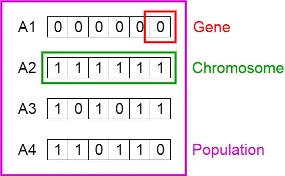
Genes are the characteristics of a individual set
chromosomes is the set of genes .Binary values are used to explain characteristics of a gene.
2.Fitness function, Fitness function determines how fit is the individual is to the best result and gives them the fitness score,And the selection is based on the fitness score.
3.Selection ,The idea of selection phase is to select the fittest individuals and allow them to pass their genes to successive generations.
4.Crossover Operator: This represents mating between individuals. Two individuals are selected using selection operator and crossover sites are chosen randomly. Then the genes at these crossover sites are exchanged thus creating a completely new individual (offspring)
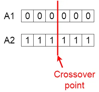
Cross over point is 3
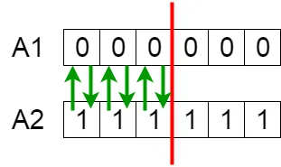
Till this point the the genes is exchanged
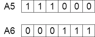
New offsprings are created
4.Mutation Operator, The key idea is to insert random genes in offspring to maintain the diversity in the population to avoid premature convergence
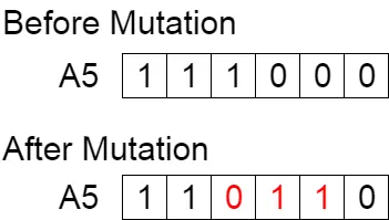
Syntax with description
finds a local unconstrained minimum, x, to the objective function, fun. nvars is the dimension (number of design variables) of fun.x to fun, subject to the linear inequalities A*x ≤ b. ga evaluates the matrix product A*x as if x is transposed (A*x').x to fun, subject to the linear equalities Aeq*x = beq and A*x ≤ b. (Set A=[] and b=[] if no linear inequalities exist.) ga evaluates the matrix product Aeq*x as if x is transposed (Aeq*x').x, so that a solution is found in the range lb ≤ x ≤ ub. (Set Aeq=[] and beq=[] if no linear equalities exist.)nonlcon. The function nonlcon accepts x and returns vectors C and Ceq, representing the nonlinear inequalities and equalities respectively. ga minimizes the fun such that C(x) ≤ 0 and Ceq(x) = 0. (Set lb=[] and ub=[] if no bounds exist.)options. (Set nonlcon=[] if no nonlinear constraints exist.) Create options using optimoptions.x = ga(fun,nvars,A,b,Aeq,beq,lb,ub,nonlcon,intcon,options)intcon take integer values.ga does not accept nonlinear equality constraints, only nonlinear inequality constraintproblem, a structure described in problem.fval, the value of the fitness function at x.exitflag, an integer identifying the reason the algorithm terminated, and output, a structure that contains output from each generation and other information about the performance of the algorithm.population, whose rows are the final population, and a vector scores, the scores of the final population.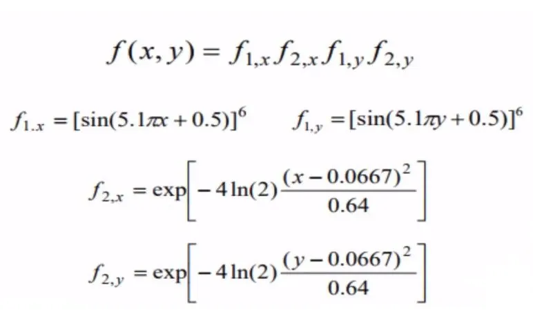
- Write a code in MATLAB to optimise the stalagmite function and find the global maxima of the function.
- Plot graphs for all 3 studies and for F maximum vs no. of iterations. Title and axes labels are a must, legends could be shown if necessary.
- Unbounded inputs
- bounded inputs
- bounded inputs with option
%The function stalagmite is created for the main program


function A = stalagmite(input_vector)

% x and y is a assigned to input_vector 1 and 2


x = input_vector(1);
y = input_vector(2);

% adding functions of stalagmite

f1 = (sin(5.1*pi*x+0.5)).^6;

f2 = exp((-4*log(2)*(x-0.0667).^2)/0.64);


f3 = (sin(5.1*pi*y+0.5)).^6;

f4 = exp((-4*log(2)*(y-0.0667).^2)/0.64);

%the negative sign is added to get the maxima

A = -(f1*f2*f3*f4);

end
x = ga(fun,nvars)
Here
× = optimal solution/ variables;
fun = Objective function;
nvars = Number of variables;
• x = ga (fun,nvars, A,B,Aeq,Beq, Ib, ub)
Here,
A, B = Linear inequality constraints
Aeq, Beq = Linear equality constraints
If there are no linear equalities and inequalities, then A, B, Aeq, Beq are set to [ ]'.
• x = ga(fun,nvars,A,B,Aeq,Beq,lb,ub, nonicon,IntCon,options)
Here,
nonlcon = Nonlinear constraints
IntCon = Integer Values
options = Optimization optionsIf there are no nonlinear constraints and integer values, the nonlcon and IntCon are set to [].
MAIN PROGRAM
clear
close all
clc


% search space id defined using linspace command

x = linspace(0,0.6,150);
y = linspace(0,0.6,150);

% number of cases is added

num_spaces = 50;

% creating 2d mesh with meshgrid command

[xx,yy] = meshgrid(x,y);

% evaluating stalagmite function

for i = 1:length(x);

   for j = 1:length(y);

    input_vector(1) = xx(i,j);

    input_vector(2) = yy(i,j);

    f(i,j) = stalagmite(input_vector);
   end
end

%-------------------------------------------------------------------------

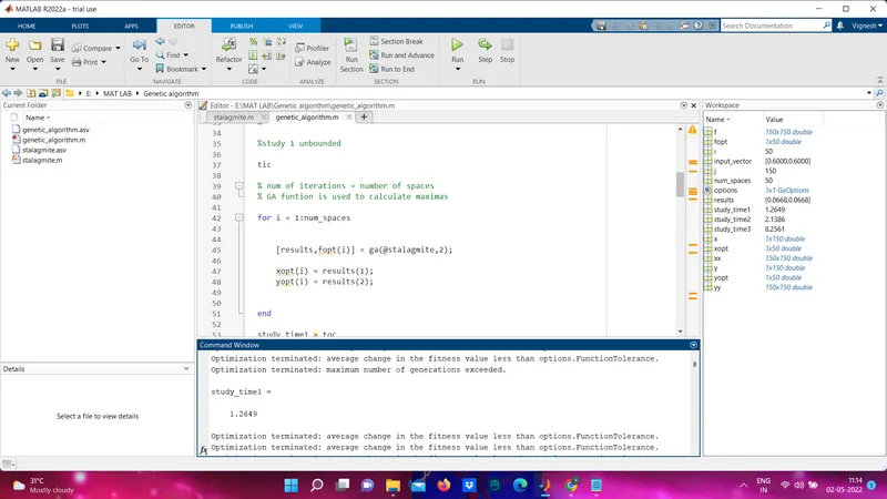
%study 1 unbounded

tic

% num of iterations = number of spaces
% GA funtion is used to calculate maximas

for i = 1:num_spaces


    [results,fopt(i)] = ga(@stalagmite,2);

    xopt(i) = results(1);
    yopt(i) = results(2);


end

study_time1 = toc

% the figure is plotted
%subplot( m , n , p ) divides the current figure into an m -by- n grid and
% creates axes in the position specified by p

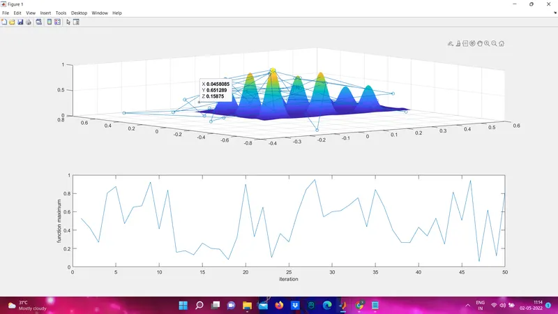
figure(1)

subplot(2,1,1)

% surf is used to produce 3d plot

surf(x,y,-f)

%shading interp varies the color in each line segment


shading interp
hold on

plot3(xopt,yopt,-fopt,'marker','o')

subplot(2,1,2)

plot(-fopt)

xlabel('iteration')
ylabel('function maximum')

%-------------------------------------------------------------------------

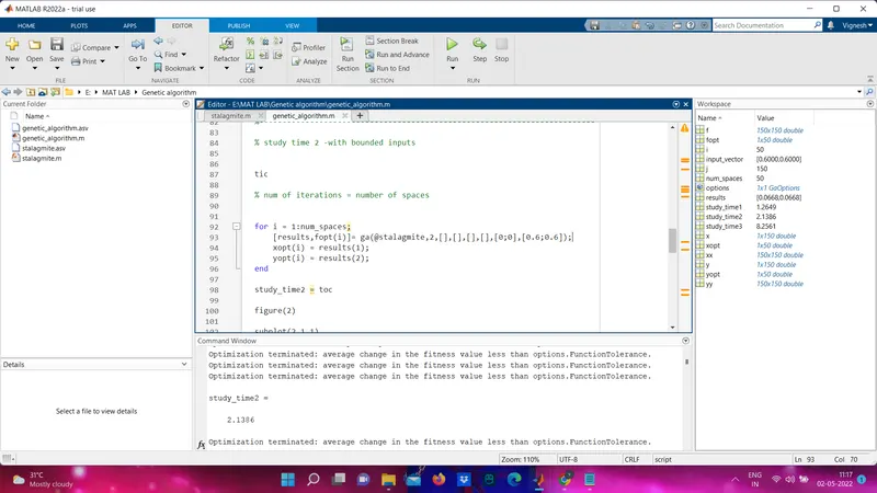
% study time 2 -with bounded inputs


tic

% num of iterations = number of spaces


for i = 1:num_spaces;
    [results,fopt(i)]= ga(@stalagmite,2,[],[],[],[],[0;0],[0.6;0.6]);
    xopt(i) = results(1);
    yopt(i) = results(2);
end

study_time2 = toc

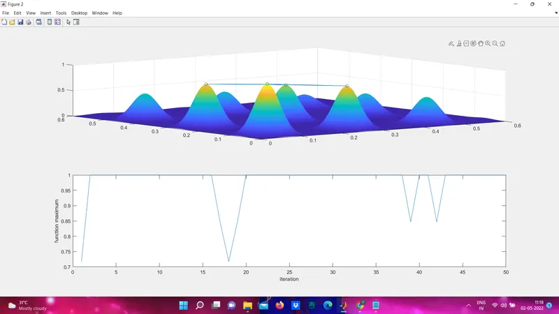
figure(2)

subplot(2,1,1)


surf(x,y,-f)

shading interp
hold on

plot3(xopt,yopt,-fopt,'marker','o')

subplot(2,1,2)

plot(-fopt)
xlabel('iteration')
ylabel('function maximum')

%--------------------------------------------------------------------------

%study time3 -bounded inputs with options
% Initial population is increases to 250

tic

options = optimoptions('ga');

options = optimoptions(options,'PopulationSize',250);

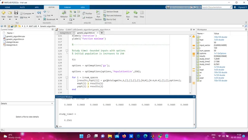
for i = 1:num_spaces
    [results,fopt(i)] = ga(@stalagmite,2,[],[],[],[],[0;0],[0.6;0.6],[],[],options);
    xopt(i) = results(1)
    yopt(i) = results(2)
end

study_time3 = toc

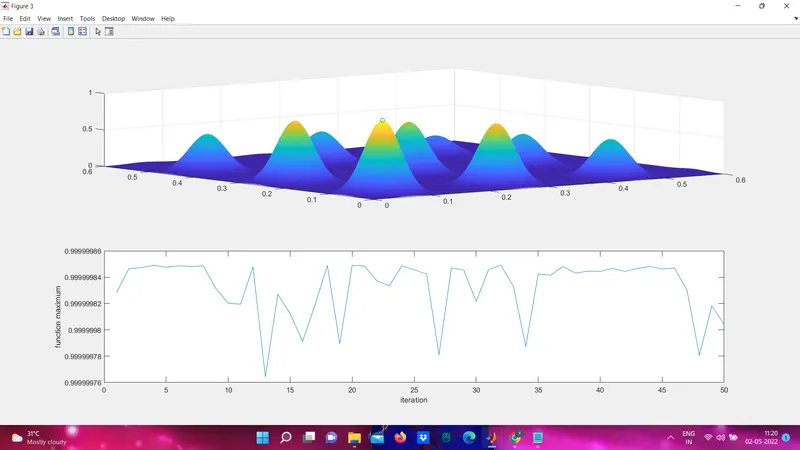
figure(3)

subplot(2,1,1)

surf(x,y,-f)

shading interp

hold on

plot3(xopt,yopt,-fopt,'marker','o');

subplot(2,1,2)

plot(-fopt)

xlabel('iteration')

ylabel('function maximum')