Week 3 - Solving second order ODEs
% second order ODE
% To solve second order we want to make the equation to first order
%this function is used to make the equation to first order
%created the function called it as dtheta_dt
%function name is ode_func and the inputs are t,theta,b,gravity,length,mass
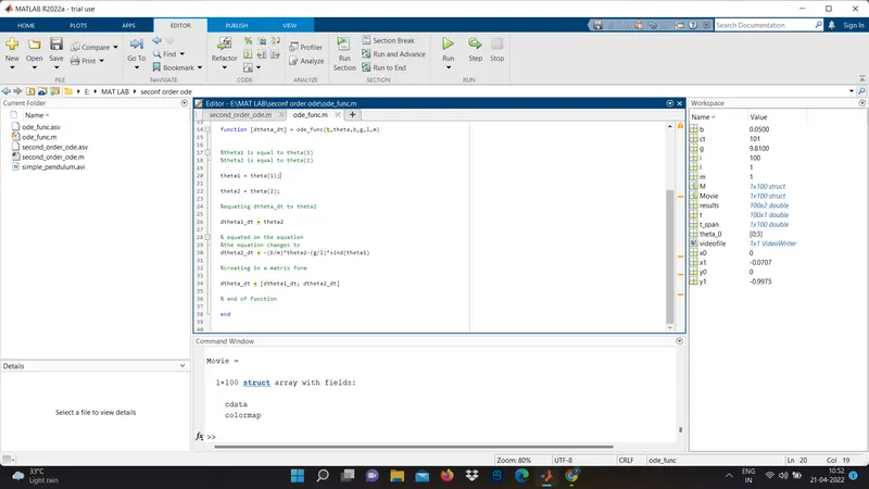
function [dtheta_dt] = ode_func(t,theta,b,g,l,m)
%theta1 is equal to theta(1)
%theta2 is equal to theta(2)
theta1 = theta(1);
theta2 = theta(2);
%equating dtheta_dt to theta2
dtheta1_dt = theta2
% equated on the equation
%the equation changes to
dtheta2_dt = -(b/m)*theta2-(g/l)*sind(theta1)
%creating in a matrix form
dtheta_dt = [dtheta1_dt; dtheta2_dt]
% end of function
end
% main program for second ode
% inputs
b = 0.05;
g = 9.81;
l = 1;
m = 1;
% displacement and initial velocity
%where displacement is zero and velocity is 3
theta_0 = [0;3];
% inputing timespan and it is from zero to 20 second with inervals of 100
%linspace is used to input 0 to 20 values with 100 intervals
t_span = linspace(0,20,100);
% t and results are tasking as the anser array for the function
% ode45 is the function used for solving first order
% ode_func is the function we created to change second order to first order
% and the result of the function is input to the ode45 function, and
% inputing t_span and initial condition theta_0
[t,results]=ode45(@(t,theta) ode_func(t,theta,b,g,l,m) ,t_span,theta_0)
% to plot graph with t and results
%we use (:,1) because we want to input from all rows and first column
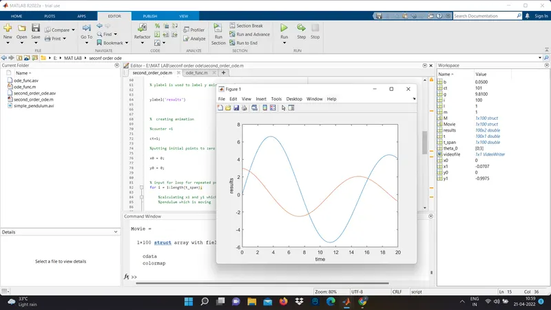
plot(t,results(:,1))
% we use hold on command to add more lines to the graph without erasing the
% existing one
hold on
% to plot graph with t and results
%we use (:,2) because we want to input from all rows and second column
plot(t,results(:,2))
%xlabel is used to name the xaxis to time
xlabel('time')
% ylabel is used to label y axis to results
ylabel('results')
% creating animation
%counter =1
ct=1;
%putting initial points to zero
x0 = 0;
y0 = 0;
% input for loop for repeated process in the length of t_span
for i = 1:length(t_span);
%calculating x1 and y1 which are the end co ordinates of simple
%pendulum which is moving
x1 =-l.*sind(results(i,1));
y1 = -l.*cosd(results(i,1))
figure(2)
% used a green beam for hanging the pendulum with width 6 and color green
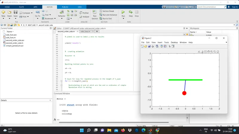
plot([-1 1],[0 0],'linewidth',6,'Color','g');
%hold on cammand is used to place another line with out erasing the
%existing one in graph
hold on
% inputing axis limits to graph
axis([-2 2 -2 2]);
% plotting the arm of pendulum with width 2 and color blue
line([x0 x1],[y0 y1],'linewidth',2,'color','b')
% ploting bob of hinch on beam and bob of pendulum
% size of hinch is 3 and color red
plot(x0,y0,'o','MarkerSize',3,'MarkerFaceColor','r')
%size of bob is 20 and color red
plot(x1,y1,'O','markersize',20,'markerface','r')
% hold off is used to stop the command
hold off
% used to get the frames to m(ct)
M(ct)=getframe(gcf);
% counter
ct = ct +1;
% to end foor loop
end
%to create movie
Movie=(M)
% to input video file name and profile
videofile= VideoWriter('simple_pendulum','uncompressed AVI');
open(videofile)
writeVideo(videofile,M)
close(videofile)
% the video is uploaded to this drive link