Week 4.1 - Genetic Algorithm
AIM:-
- Write a code in MATLAB to optimise the stalagmite function and find the global maxima of the function.
- Clearly expalin the concept of genetic algorithm in your own words and also explain the syntax for ga in MATLAB in your report.
- Make sure that your code gives the same output, even if it is made to run several times.
- Plot graphs for all 3 studies and for F maximum vs no. of iterations. Title and axes labels are a must, legends could be shown if necessary.
BASIC THEORY-
A genetic algorithm is a search heuristic that is inspired by Charles Darwin’s theory of natural evolution. This algorithm reflects the process of natural selection where the fittest individuals are selected for reproduction in order to produce offspring of the next generation.
Genetic algorithms simulate the process of natural selection which means those species who can adapt to changes in their environment are able to survive and reproduce and go to next generation. In simple words, they simulate “survival of the fittest” among individual of consecutive generation for solving a problem. Each generation consist of a population of individuals and each individual represents a point in search space and possible solution. Each individual is represented as a string of character/integer/float/bits. This string is analogous to the Chromosome.
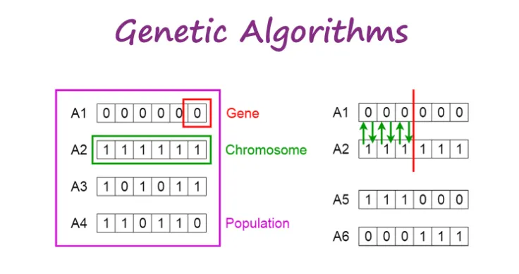
The process of natural selection starts with the selection of fittest individuals from a population. They produce offspring which inherit the characteristics of the parents and will be added to the next generation. If parents have better fitness, their offspring will be better than parents and have a better chance at surviving. This process keeps on iterating and at the end, a generation with the fittest individuals will be found.
This notion can be applied for a search problem. We consider a set of solutions for a problem and select the set of best ones out of them.
Five phases are considered in a genetic algorithm.
- Initial population
- Fitness function
- Selection
- Crossover
- Mutation
Initial population
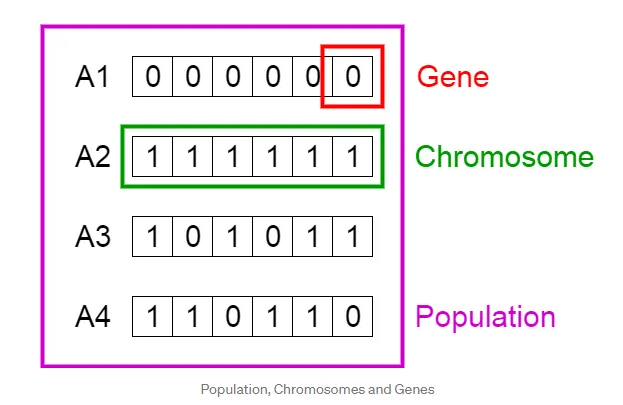
The process begins with a set of individuals which is called a Population. Each individual is a solution to the problem you want to solve.An individual is characterized by a set of parameters (variables) known as Genes. Genes are joined into a string to form a Chromosome (solution).In a genetic algorithm, the set of genes of an individual is represented using a string, in terms of an alphabet. Usually, binary values are used (string of 1s and 0s). We say that we encode the genes in a chromosome.
Fitness function
The fitness function determines how fit an individual is (the ability of an individual to compete with other individuals). It gives a fitness score to each individual. The probability that an individual will be selected for reproduction is based on its fitness score.
Selection
The idea of selection phase is to select the fittest individuals and let them pass their genes to the next generation.Two pairs of individuals (parents) are selected based on their fitness scores. Individuals with high fitness have more chance to be selected for reproduction.
Crossover
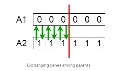
Crossover is the most significant phase in a genetic algorithm. For each pair of parents to be mated, a crossover point is chosen at random from within the genes.
For example, consider the crossover point to be 3 as shown below.
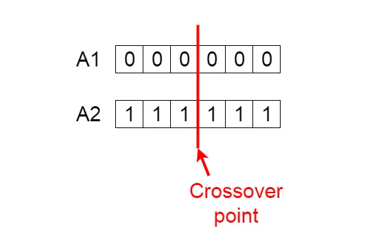
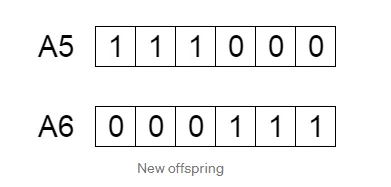
Offspring are created by exchanging the genes of parents among themselves until the crossover point is reached.
The new offspring are added to the population.
Mutation
In certain new offspring formed, some of their genes can be subjected to a mutation with a low random probability. This implies that some of the bits in the bit string can be flipped.
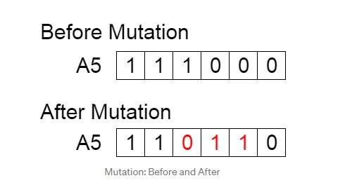
Mutation occurs to maintain diversity within the population and prevent premature convergence.
SYNTAX FOR GA:-
x = ga(fun,nvars)-x = ga(fun,nvars,A,b)x = ga(fun,nvars,A,b,Aeq,beq)x = ga(fun,nvars,A,b,Aeq,beq,lb,ub)x = ga(fun,nvars,A,b,Aeq,beq,lb,ub,nonlcon)x = ga(fun,nvars,A,b,Aeq,beq,lb,ub,nonlcon,options)x = ga(fun,nvars,A,b,Aeq,beq,lb,ub,nonlcon,intcon)x = ga(fun,nvars,A,b,Aeq,beq,lb,ub,nonlcon,intcon,options)x = ga(problem)[x,fval] = ga(___)[x,fval,exitflag,output] = ga(___)[x,fval,exitflag,output,population,scores] = ga(___)
where,
x = ga(fun,nvars)x, to the objective function, fun. nvars is the dimension (number of design variables) of fun.
x = ga(fun,nvars,A,b)x to fun, subject to the linear inequalities A*x ≤ b. ga evaluates the matrix product A*x as if x is transposed (A*x').
x = ga(fun,nvars,A,b,Aeq,beq)x to fun, subject to the linear equalities Aeq*x = beq and A*x ≤ b. (Set A=[] and b=[] if no linear inequalities exist.) ga evaluates the matrix product Aeq*x as if x is transposed (Aeq*x').
x = ga(fun,nvars,A,b,Aeq,beq,lb,ub)x, so that a solution is found in the range lb ≤ x ≤ ub. (Set Aeq=[] and beq=[] if no linear equalities exist.)
x = ga(fun,nvars,A,b,Aeq,beq,lb,ub,nonlcon)nonlcon. The function nonlcon accepts x and returns vectors C and Ceq, representing the nonlinear inequalities and equalities respectively. ga minimizes the fun such that C(x) ≤ 0 and Ceq(x) = 0. (Set lb=[] and ub=[] if no bounds exist.)
x = ga(fun,nvars,A,b,Aeq,beq,lb,ub,nonlcon,options)options. (Set nonlcon=[] if no nonlinear constraints exist.) Create options using optimoptions.
x = ga(fun,nvars,A,b,Aeq,beq,lb,ub,nonlcon,intcon)x = ga(fun,nvars,A,b,Aeq,beq,lb,ub,nonlcon,intcon,options)intcon take integer values.
x = ga(problem)problem, a structure described in problem.
[, for any previous input arguments, also returns x,fval] = ga(___)fval, the value of the fitness function at x.
[ also returns x,fval,exitflag,output] = ga(___)exitflag, an integer identifying the reason the algorithm terminated, and output, a structure that contains output from each generation and other information about the performance of the algorithm.
[ also returns a matrix x,fval,exitflag,output,population,scores] = ga(___)population, whose rows are the final population, and a vector scores, the scores of the final population.
STALAGMITE FUNCTION:-
A stalagmite is a type of speleothem that rises from the floor of a limestone cave due to the dripping of mineralized solutions and the deposition of calcium carbonate.
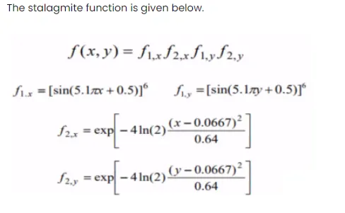
STALAGMITE FUNCTION CODE
function A =stalagmite_function(input_vector)
x=input_vector(1);
y=input_vector(2);
f1=(sin(5.1*pi*x+0.5)).^6;
f2=(sin(5.1*pi*y+0.5)).^6;
f3=exp((((x-0.0667).^2)/0.64)*(-4*log(2)));
f4=exp((((y-0.0667).^2)/0.64)*(-4*log(2)));
A=-(f1*f2*f3*f4);
end
MAIN PROGRAM CODE
close all
clear all
clc
%input
x=linspace(0,0.6,150);
y=linspace(0,0.6,150);
num_spaces=50
%forming 2d array
[xx yy]=meshgrid(x,y);
for i=1:length(x)
for j=1:length(y);
input_vector(1)=xx(i,j);
input_vector(2)=yy(i,j);
f(i,j)=stalagmite_function(input_vector);
end
end
%study1 unbounded
tic
for i=1:num_spaces
[result,fopt(i)]=ga(@stalagmite_function,2)
xopt(i)=result(1)
yopt(i)=result(2)
end
study_time1=toc
%plotting
figure(1)
subplot(2,1,1)
surf(x,y,-f)
shading interp
hold on
plot3(xopt,yopt,-fopt,'marker','o')
subplot(2,1,2)
plot(-fopt)
xlabel('iteration')
ylabel('function maximum')
%study 2- unbounded
tic
for i=1:num_spaces
[result,fopt(i)]=ga(@stalagmite_function,2,[],[],[],[],[0;0],[0.6;0.6])
xopt(i)=result(1)
yopt(i)=result(2)
end
study_time2=toc
%plotting
figure(2)
subplot(2,1,1)
surf(x,y,-f)
shading interp
hold on
plot3(xopt,yopt,-fopt,'marker','o')
subplot(2,1,2)
plot(-fopt)
xlabel('iteration')
ylabel('function maximum')
%study3-incresed initial population
tic
options=optimoptions('ga')
options=optimoptions(options,'populationsize',250)
for i=1:num_spaces
[result,fopt(i)]=ga(@stalagmite_function,2,[],[],[],[],[0;0],[0.6;0.6],[],[],options)
xopt(i)=result(1)
yopt(i)=result(2)
end
study_time3=toc
figure(3)
subplot(2,1,1)
surf(x,y,-f)
shading interp
hold on
plot3(xopt,yopt,-fopt,'marker','o')
subplot(2,1,2)
plot(-fopt)
xlabel('iteration')
ylabel('function maximum')
EXPLANATION OF PROGRAM
Part 1:-
x=linspace(0,0.6,150);
y=linspace(0,0.6,150);
num_spaces=50
%forming 2d array
[xx yy]=meshgrid(x,y);
for i=1:length(x)
for j=1:length(y);
input_vector(1)=xx(i,j);
input_vector(2)=yy(i,j);
f(i,j)=stalagmite_function(input_vector);
end
end
- Initialize values for x and y by taking 150 values between 0 to 0.6.
- we have consider number of iteration to perform using num_spaces command
- our requirement is 3D plot so, we have taken 2D array of x and y using meshgrid() command.
- we have stored values of x and y in input_vector array. its used during calling of stalagmite function.
- Now to get maxima,we have made some changes in stalagmite function. 'ga' always give minimum value as a output, so we have taken '-f' as output.
- Nasted for function is used here.
Part 2:-
%study1 unbounded
tic
for i=1:num_spaces
[result,fopt(i)]=ga(@stalagmite_function,2)
xopt(i)=result(1)
yopt(i)=result(2)
end
study_time1=toc
%plotting
figure(1)
subplot(2,1,1)
surf(x,y,-f)
shading interp
hold on
plot3(xopt,yopt,-fopt,'marker','o')
subplot(2,1,2)
plot(-fopt)
xlabel('iteration')
ylabel('function maximum')
- Now lets start our first case study,firstly we have taken no.of iteration is equal to num_spaces.
- 'ga' function is used to to calculate the maxima.its outputs are stored in result() which contains maxima.
- Here fopt is contain the value of which maxima is obtained.
- As we required 3D plot, we have used surf() function. Plot3() command is used to plot xopt,yopt and -fopt.
- Here -fopt fuction will visualise the optimum value at each iteration.
- tic-toc function is used to get time taken to complete cycle
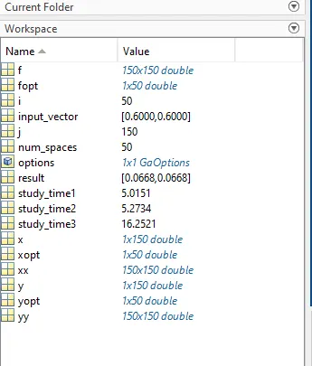
After this we have run the code and our output is displayed as,
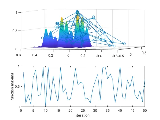
After 1st case study, we have output which showing that optimum values are went outside from value of x and y. so, our result is falling away from stalagmite surface. According to all this result, we are failed to get the global maxima in this case,out study time is 4.5714 s.
Now,in second case study we have taken bounded values. Lower and upper bounds of x and y are specified,the ga is initiated with random population only.
ERROR AND SOLUTION:-
1)

SOLUTION- in ga function i have used 'stalagmite' word to give input. however in out code i have used 'stalagmite_function'. so after making this correct my code is run properly.
2)
solution-I have written marker'. Here i had missed upper semicolon. so i have correct it as 'marker' later.
Part 2:-
%study 2- unbounded
tic
for i=1:num_spaces
[result,fopt(i)]=ga(@stalagmite_function,2,[],[],[],[],[0;0],[0.6;0.6])
xopt(i)=result(1)
yopt(i)=result(2)
end
study_time2=toc
%plotting
figure(2)
subplot(2,1,1)
surf(x,y,-f)
shading interp
hold on
plot3(xopt,yopt,-fopt,'marker','o')
subplot(2,1,2)
plot(-fopt)
xlabel('iteration')
ylabel('function maximum')
- Here we have done some as our previous case, we have stored result into xopt, yopt and surf.
- Here also we have used plot3 command to plot xopt,yopt and -fopt.
- lets plot the fopt function so that we can visualise the optimum value at each iteration.
- tic-tac command is used to get time for complete cycle.
after running this code, our result will displayed as below
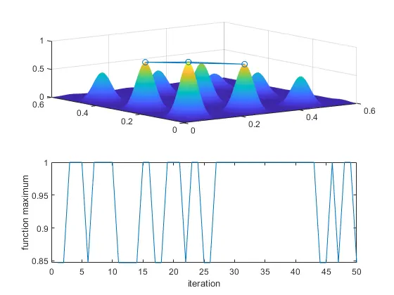
As per above result, optimum values are within the limit and it could not give us the exact maxima values. This case study has taken 5.5244 s time and its more than previous one.
Part:-3
%study3-incresed initial population
tic
options=optimoptions('ga')
options=optimoptions(options,'populationsize',250)
for i=1:num_spaces
[result,fopt(i)]=ga(@stalagmite_function,2,[],[],[],[],[0;0],[0.6;0.6],[],[],options)
xopt(i)=result(1)
yopt(i)=result(2)
end
study_time3=toc
figure(3)
subplot(2,1,1)
surf(x,y,-f)
shading interp
hold on
plot3(xopt,yopt,-fopt,'marker','o')
subplot(2,1,2)
plot(-fopt)
xlabel('iteration')
ylabel('function maximum')
EXPLANATION:-
- Here in this case, to set a initial population we have used 'optimumoptions' and get our value of 'populationsize' to 250.
- Now we store the result into xopt, yopt as previous we need to plot the surf function to get 3D plot.
- Plot3 command is used to make plot of xopt, yopt and -fopt to plot the optimum maxima.
- fopt function is used for visualise the optimum values at each iteration.
- tic-toc command is used to get the time required to complete cycle.
After running this code, the output will displayed as
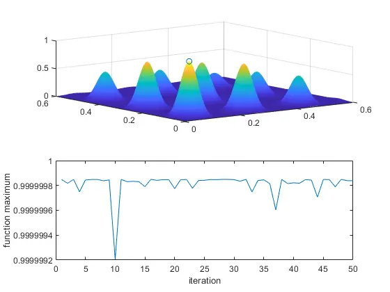
Time execution for this case study is more as compared with previous two. In this case we are sucessful to findout correct maxima for the stalagmite function.
As a result, we have findout that when we increased initial population size of the ga, we will get better accuracy of the algorithm. Time taken for this case study is 16.5878s.
FINAL OUTPUT:-