Project 2 - Rankine cycle Simulator
OO
OBJECTIVE:-
- Create a Rankine Cycle Simulator using OCTAVE/MATLAB.
- Your code should calculate the state points of the Rankine Cycle (any type of your choice) based on user inputs.
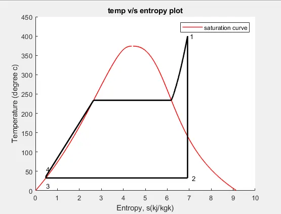
- Then, plot the corresponding T-s and h-s plots for the given set of inputs. Title and axes labels are a must, while legends could be used if necessary.
- The presentation of your code will be taken into consideration while grading. Labelling sections of your code using comments is appreciated.
- Attach a report explaining the working of a rankine cycle simulator and also the research done by you.
BASIC CONCEPT:-
Basic Cycle
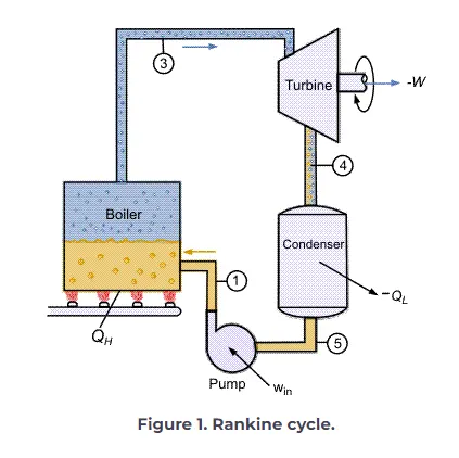
The Rankine cycle is the fundamental operating cycle of all power plants where an operating fluid is continuously evaporated and condensed. The selection of operating fluid depends mainly on the available temperature range. Figure 1 shows the idealized Rankine cycle.
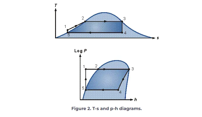
The pressure-enthalpy (p-h) and temperature-entropy (T-s) diagrams of this cycle are given in Figure 2. The Rankine cycle operates in the following steps:
-
1-2-3 Isobaric Heat Transfer. High pressure liquid enters the boiler from the feed pump (1) and is heated to the saturation temperature (2). Further addition of energy causes evaporation of the liquid until it is fully converted to saturated steam (3).
-
3-4 Isentropic Expansion. The vapor is expanded in the turbine, thus producing work which may be converted to electricity. In practice, the expansion is limited by the temperature of the cooling medium and by the erosion of the turbine blades by liquid entrainment in the vapor stream as the process moves further into the two-phase region. Exit vapor qualities should be greater than 90%.
-
4-5 Isobaric Heat Rejection. The vapor-liquid mixture leaving the turbine (4) is condensed at low pressure, usually in a surface condenser using cooling water. In well designed and maintained condensers, the pressure of the vapor is well below atmospheric pressure, approaching the saturation pressure of the operating fluid at the cooling water temperature.
-
5-1 Isentropic Compression. The pressure of the condensate is raised in the feed pump. Because of the low specific volume of liquids, the pump work is relatively small and often neglected in thermodynamic calculations.
The efficiency of power cycles is defined as
Values of heat and work can be determined by applying the First Law of Thermodynamics to each step. The steam quality x at the turbine outlet is determined from the assumption of isentropic expansion, i.e.,
where is the entropy of vapor and Si* the entropy of liquid.
Required Inputs:
Turbine Inlet temperature = 400° C
Turbine Inlet Pressure = 30 bars
Turbine Outlet Pressure = 0.05 bars = Condenser Inlet Pressure
MAIN PROGRAM:-
%rankine cycle simulator
clear all
close all
clc
disp('Rankine cycle');
disp('1-2 Iscentropic expansion in the turbine');
disp('2-3 constant pressure heat removal in condenser');
disp('3-4 iscentropic compression in the pump')
disp('4-1 constant pressure heat addition in the boiler');
%Obtaining input data
T1=input('value of temperature at turbine inlet, T1(in degree c)= ');
p1=input('value of pressure at turbine inlet, p1(in bar )= ');
p2=input('value of pressure at condenser inlet, p2(in bar )= ');
%extracting data variable of point1
h1=XSteam('h_pT',p1,T1); %extracting enthalpy at point1
s1=XSteam('s_pT',p1,T1); %extracting entropy at point1
%extracting data variable of point2
s2=s1; %iscentropic expansion
sf2=XSteam('sL_p',p2); %saturated liquid entropy
sg2=XSteam('sV_p',p2); %saturated vapour entropy
x2=(s2-sf2)/(sg2-sf2);
hf2=XSteam('hL_p',p2);
hg2=XSteam('hL_p',p2);
h2=hf2+(x2*(hg2-hf2));
%extracting data variable of point3
p3=p2
s3=XSteam('sL_p',p3);
h3=XSteam('hL_p',p3);
%extracting data variable of point4
s4=s3;
p4=p1;
%workdone by turbine
Wt=h1-h2;
%workdone by pump
V3=XSteam('VL_p',p3);
Wp=V3*(p4-p3)*100;
h4=h3+Wp;
%net work
Wnet=Wt-Wp;
%heat in of the system
Qin=h1-h4;
%heat out of the system
Qout=h2-h3;
%thermal efficieny
eff=(Wnet/Qin)*100;
%specific steam consumption
%ssc=mass flow rate/power
ssc=(3600/Wnet);
%calculating temperature at state points
T3=XSteam('Tsat_p',p3);
T2=T3;
Cp4=XSteam('Cp_ps',p4,s4);
Cv4=XSteam('Cv_ps',p4,s4);
k=Cp4/Cv4;
T4=T3/((p3/p4)^((k-1)/k));
%calculating temperature,entropy,enthalpy at the vapout and liquid
T6=XSteam('Tsat_p',p1);
s5=XSteam('sL_p',p1);
s6=XSteam('sV_p',p1);
h5=XSteam('hL_p',p1);
h6=XSteam('hV_p',p1);
T5=T6;
%plotting saturation curve
T=linspace(1,380,1000);
for i=1:length(T)
sf(i)=XSteam('sL_T',T(i));
sg(i)=XSteam('sV_T',T(i));
hf(i)=XSteam('hL_T',T(i));
hg(i)=XSteam('hV_T',T(i));
end
%Plotting T-s diagram
figure(1)
hold on
plot(sf,T,'r','linewidth',1)
plot(sg,T,'r','linewidth',1)
plot([s1 s2],[T1 T2],'k','linewidth',2)
plot([s2 s3],[T2 T3],'k','linewidth',2)
plot([s3 s4],[T3 T4],'k','linewidth',2)
plot([s4 s5],[T4 T5],'k','linewidth',2)
plot([s5 s6],[T5 T6],'k','linewidth',2)
sc1=linspace(s6,s1,1000);
for i=1:length(sc1)
Tc1(i)=XSteam('T_ps',p1,sc1(i));
end
plot(sc1,Tc1,'k','linewidth',2)
text(s1+0.1,T1,'1')
text(s2+0.2,T2,'2')
text(s3,T3-20,'3')
text(s4,T4+20,'4')
title('temp v/s entropy plot')
xlabel('Entropy, s(kj/kgk)')
ylabel('Temperature (degree c)')
legend('saturation curve')
%displaying results
disp('Result')
fprintf('At state point 1:n');
fprintf('p1:%8.3f barn',p1);
fprintf('T1:%8.3f Cn',T1);
fprintf('h1:%8.3f kj/kgn',h1);
fprintf('s1:%8.3f kj/kgknn',s1);
fprintf('At state point 2:n');
fprintf('p2:%8.3f barn',p2);
fprintf('T2:%8.3f Cn',T2);
fprintf('h2:%8.3f kj/kgn',h2);
fprintf('s2:%8.3f kj/kgknn',s2);
fprintf('At state point 3:n');
fprintf('p3:%8.3f barn',p3);
fprintf('T3:%8.3f Cn',T3);
fprintf('h3:%8.3f kj/kgn',h3);
fprintf('s3:%8.3f kj/kgknn',s3);
fprintf('At state point 4:n');
fprintf('p4:%8.3f barn',p4);
fprintf('T4:%8.3f Cn',T4);
fprintf('h4:%8.3f kj/kgn',h4);
fprintf('s4:%8.3f kj/kgknn',s4);
fprintf('Turbine work:%8.3f kj/kgn',Wt);
fprintf('Pump work:%8.3f kj/kgn',Wp);
fprintf('Wnet:%8.3f kj/kgn',Wnet);
fprintf('Efficiency:%8.3f percent n',eff);
fprintf('ssc : %8.3f kj/kWh',ssc);
ERRORS:-


OUTPUT:-
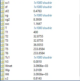
OUTPUT ON COMMENT BOX:-
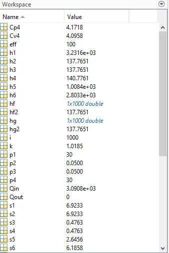
At state point 1:np1: 30.000 barnT1: 400.000 Cnh1:3231.571 kj/kgns1: 6.923 kj/kgknnAt state point 2:np2: 0.050 bar /fT2: 32.875 Cn /fh2: 137.765 kj/kgn /fs2: 6.923 kj/kgknn /fAt state point 3:np3: 0.050 barnT3: 32.875 Cnh3: 137.765 kj/kgns3: 0.476 kj/kgknnAt state point 4:np4: 30.000 barnT4: 36.935 Cnh4: 140.776 kj/kgns4: 0.476 kj/kgknnTurbine work:3093.806 kj/kgnPump work: 3.011 kj/kgnWnet:3090.795 kj/kgnEfficiency: 100.000 percent nssc : 1.165 kj/kWh>>
>>
REFEFARANCE:-
1) https://www.thermopedia.com/content/1072/
2) https://energyeducation.ca/encyclopedia/Rankine_cycle
3) https://www.mathworks.com/help/physmod/simscape/ug/rankine-cycle-steam-turbine.html
CODE EXPLANATION:-
XSteam data is used to extract steam and water properties of enthalpy,entropy at specific pressure and temperature for saturated liquid, saturated vapour conditions etc.
This program requires the input of pressure in bar at state point 1 as a turbine input temperature at same point in degree cel. and temperature at condenser input in degree cel.
With the help of these inlets and from xstream data, the program calculates all the state points of the rankine cycle.
The steam data is works as h1=xsteam(h_pt,p1,T1) returns the enthalpy of water at given pressure and temp. in bar and degree c respectively.
As we extract data, we have to used thermodyanic relations to findout state points and extract there data from xsteam.
sf and sg & hf and hg, where f and g are saturated liquid(f) and saturated vapour(g) respectively.
Using thermodyanic relation we have to calculated net work, workdone by turbine,workdone to run run the pump. heat in and heat out are calculated.
Then, specific steam consumption(ssc) and efficiency of the rankine cycle are calculated.
T,s and h extracted at vapour and liquid line for plotting purpose, after 4th point for the variation you observe in the plot.
Saturation curve is plotted in red for saturated liquid and gas
Plot of T v/s s and h v/s s is created from all points obtained from the program.
Result are displayed in command window.