Week 4.1 - Genetic Algorithm
GENETIC ALGORITHM
AIM:-to optimise the statalgmite function and the global maxima of the function.
OBJECTIVE:- explainig the concept of genetic algorithm and also explain the syntax of GA in matlab.
INTRODUCTION:-A genetic algorithm is a search experiential that is stimulated by charles derwins's theory of natural reproduction .this algorithm reproduces the process of natural selection where the appropriate ibndividuals are selected for reproduction in order top produce odfspring of the next generation.
the genetic algorithm is a technique for solving both constraints and unconstrained optimization problems that atre based on natural selection,the process that drives biological evolution.the geneticd algorithm constantly modifies the population size of individual solution.
PHASES OF GENETIC ALGORITHM
Initialisation of population:- the codes generates its randon population of defined size and from that population the codes evaluates the fitness of the members of the popuplation according to which ot forms now population basd on number of iterations performed.
Fitness of function:-it is that function which we have to optimise.optimization is done the help of generations which have been found by theb code accordance with the fitness value of each member generated,these fitness values are used for the reproduction of the children.
Selection:-the idea of selection phase is to select the fittest individuals and let them pass their genes to the next generation.the main goal of this phase id to find the region where chances of getting the best solution are more.
Cross-over:-It is the process of taking two parents and producing the child from them by interchanging the genes.there are many ways to do cross-over opertions.
Mutation:-Mutation is carried out to maintain the genetic diversity from one generation of a population of chromosomes to t the next.In this process the genes will be replaced by some random integers.
usually, total genes=no.of genes*no of population.
eg-2*5=10
hence, the random values will be generated between 1 to 1o(total gene).
if mutation is not performed the chromosomes will become too similar to each other,convergance takes place soon and results in local minima.
Where is GA used?
Genetics algorithm are primarily used in optimization problems of various kinds,but they are frequently used in other applications areas as well.
the areas in which the genetic algorithm is used are given below:
optimization:-genetic algorithm are most commonly used in optimization problems wherein we have to maximize or minimize a given objective function value under a given set of constraints.
Economics:-GAs are also used to characterise various economic models like the cobweb model,asset pricing etc.
image processing :-GAs are used for variuos digital image processing(DIP) tasks as well like dense pixel matching.
SYNTAX OF GA
[x,fval,exitflag,output,population,scores]=ga(func,nvars,A,B,Aeb,Beq,lb,ub,nonlcon,intcon,options)
where, x =optimum solution
exitflag = reason ga stopped
output = information about optimization process
population = final population
scores = final scores
fun = fitness function
nvars = no. of variables
A,b = linear inequality constraints
Aeq,Beq = linear equality constraints
lb = lower bound(limit)
ub = upper bound (limit)
nonlcon = used for non-linear constraints
intcon = to get solution in integer
options = to set population size minimize with non-default options.
WRITING A PROGRAM IN MATLAB
using the formula as given below,
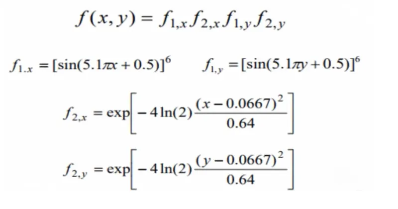
code in matlab,
function f = satalgmite_fun(input)
x = input(1);
y = input(2);
f1x = (sin(((5.1*pi).*x)+0.5)).^6;
f1y = (sin(((5.1*pi).*y)+0.5)).^6;

f2x = exp((((x-0.0667).^2).*(-4*log(2)))./0.64);
f2y = exp((((y-0.0667).^2).*(-4*log(2)))./0.64);

f = -f1x*f1y*f2x*f2y;

end
wriring a code to plot,
clear all
close all
clc

%defining  search space
x = linspace(0,0.6,150);
y = linspace(0,0.6,150);

%creating a 2dimensional mesh
[xx,yy] = meshgrid(x,y);

num_cases =50;

%evaluating a stalagmite function

for i = 1:length(xx)
    for j = 1:length(yy)
        input_vector(1) = xx(i,j);
        input_vector(2) = yy(i,j);
        f(i,j) = stalagmite_function(input_vector);
    end
end

surf(xx,yy,f);
shading interp

[x, fval] = ga(@stalagmite_function,2)
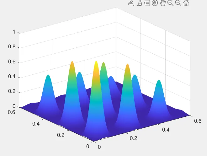
hence,the plot is created
1-STATISTICAL STUDIES WITHOUT BOUNDATION
>Evaluating the optimum value of fitness function at each iterationsand calculating it using the syntax.
writing a program for study of unbounded points.
clear all
close all
clc

%defining  search space
x = linspace(0,0.6,150);
y = linspace(0,0.6,150);

%creating a 2dimensional mesh
[xx,yy] = meshgrid(x,y);

num_cases =50;

%evaluating a stalagmite function

for i = 1:length(xx)
    for j = 1:length(yy)
        input_vector(1) = xx(i,j);
        input_vector(2) = yy(i,j);
        f(i,j) = stalagmite_function(input_vector);
    end
end

surfc(x,y,f);
%study 1
tic
for i=1:num_cases

    [inputs,fopt(i)]= ga(@stalagmite_function,2);
    xopt(i)=inputs(1);
    yopt(i)=inputs(2);
end
fopt =-fopt;
study_time=toc    %displaying the time taken evaluate

%plottong the graph
figure(1)
subplot(2,1,1)
hold on
surfc(x, y, -f);
shading interp
plot3(xopt,yopt,fopt,'marker','o','markersize',5,'markerfacecolor','r')
title('unbounded inputs')
subplot(2,1,2)
plot(fopt)
xlabel('iterations')
ylabel('function minimum')
hence,the plot is created
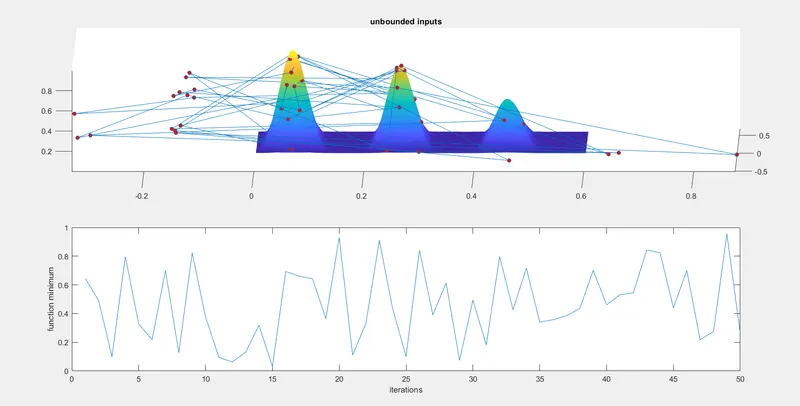
the study time for optimising the function is
4.2270
from the above figure it is clear that the results are not that much accurate and
giving a lot of variation in optimizing the function.
2-STATISTICAL STUDY WITH BOUNDATION
The difference over here is providing the upper limits and lower limits in the ga
so that the search space is reduced with upper and lower limit boundary.
Writing a program in Matlab
clear all
close all
clc

%defining  search space
x = linspace(0,0.6,150);
y = linspace(0,0.6,150);

%creating a 2dimensional mesh
[xx,yy] = meshgrid(x,y);

num_cases =50;

%evaluating a stalagmite function

for i = 1:length(xx)
    for j = 1:length(yy)
        input_vector(1) = xx(i,j);
        input_vector(2) = yy(i,j);
        f(i,j) = stalagmite_function(input_vector);
    end
end

surfc(x,y,f);

tic
%study 2-statistics with upper and lower bounds.

for i = 1:num_cases
    [inputs,fopt(i)] = ga(@stalagmite_function,2,[],[],[],[],[0,0],[1,1]);

    xopt(i) = inputs(1);
    yopt(i) = inputs(2);

end
fopt = -fopt
study_time = toc

figure(2)
subplot(2,1,1)
hold on
surfc(x,y,-f)
shading interp
plot3(xopt,yopt,fopt,'marker','o','markersize',5,'markerfacecolor','r')
title('Bounded inputs')
subplot(2,1,2)
plot(fopt)
xlabel('iteration')
ylabel('function minimum')
the plot is given below,
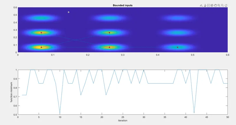
the study time for optimisinfgthe function is
6.7363
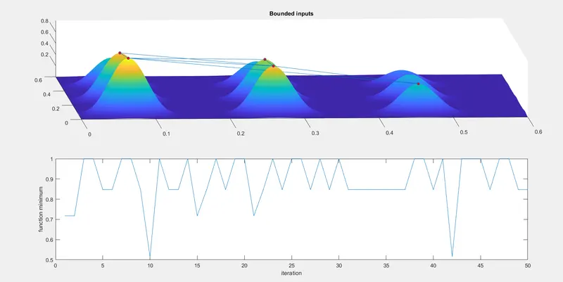
hence,it is clearly seen from the above that after providing the boundary limits
the variation in the optimum value of the function has reduced.
3-STATISTICAL STUDY WITH INCREASE IN SIZE OF POPULATION
In this study using the 'optimoptions' command to increase the size in the population.
it will increase the possibilities of finding the better fitness if function.
Writing a program in Matlab,
clear all
close all
clc

%defining  search space
x = linspace(0,0.6,150);
y = linspace(0,0.6,150);

%creating a 2dimensional mesh
[xx,yy] = meshgrid(x,y);

num_cases =50;

%evaluating a stalagmite function

for i = 1:length(xx)
    for j = 1:length(yy)
        input_vector(1) = xx(i,j);
        input_vector(2) = yy(i,j);
        f(i,j) = stalagmite_function(input_vector);
    end
end

surfc(x,y,f);

%study 3- increasing the GA iterations
options = optimoptions('ga');
options = optimoptions(options,'PopulationSize',300);

tic
for i = 1:num_cases
    [inputs,fopt(i)] = ga(@stalagmite_function,2,[],[],[],[],[0;0],[1;1],[],[],options);
xopt(i) = inputs(1);
yopt(i) = inputs(2);

end
fopt = -fopt
study_time = toc

figure(3)
subplot(2,1,1)
hold on
surfc(x,y,-f)
shading interp
plot3(xopt,yopt,fopt,'marker','o','markersize',5,'markerfacecolor','r');
title('Bounded inputs with modified population size')
subplot(2,1,2)
plot(fopt)
xlabel('Iterations')
ylabel('function minimum')
the plot is shown below,
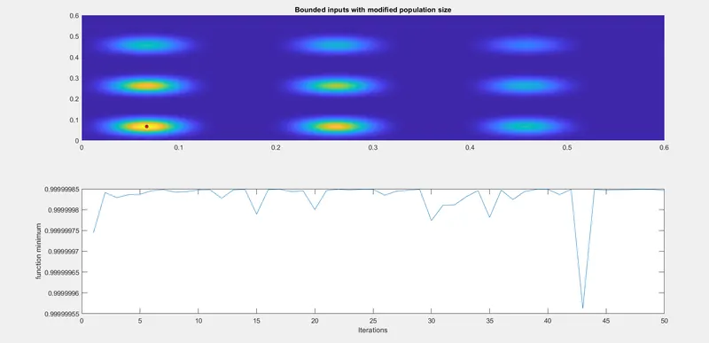
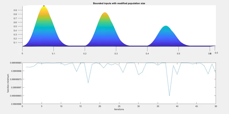
it is clearly seen in the above case that the variation has changed to a large extent.
the study_time for optimising the function is
15.4720
ALL THE CODES , COMMANDS AND RESULTS ARE ATTACHED.