Week 4.1 - Genetic Algorithm
AIM:-
To optimize the stalagmite function and find the global maxima of the function by using matlab.
THEORY:-
- What is optimization? Various optimization techniques.
- What is genetic algorithm?
- How genetic algorithm work? Where we use genetic algorithm?
Optimization: The process in which there are various alternatives and the selection of best alternatives among them all is an optimization.
There are two optimization methods.
(a) Deterministic Algorithms.
They use specific rules for moving one solution to other. These
algorithms are in use to suite some times and have been
successfully applied for many engineering design problems.
(b) Stochastic Algorithms.
The stochastic algorithms are in nature with probabilistic
translation rules. These are gaining popularity due to certain
properties which deterministic algorithms do not have.
Genetic Algorithm:
The genetic algorithm is a method for solving both constrained and unconstrained optimization problems that is based on natural selection, the process that drives biological evolution. The genetic algorithm repeatedly modifies a population of individual solutions. At each step, the genetic algorithm selects individuals from the current population to be parents and uses them to produce the children for the next generation. Over successive generations, the population "evolves" toward an optimal solution. You can apply the genetic algorithm to solve a variety of optimization problems that are not well suited for standard optimization algorithms, including problems in which the objective function is discontinuous, nondifferentiable, stochastic, or highly nonlinear. The genetic algorithm can address problems of mixed integer programming, where some components are restricted to be integer-valued.
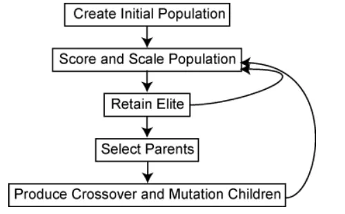
This flow chart outlines the main algorithmic steps.
How the Genetic Algorithm Works
Outline of the Algorithm
The following outline summarizes how the genetic algorithm works:
-
The algorithm begins by creating a random initial population.
-
The algorithm then creates a sequence of new populations. At each step, the algorithm uses the individuals in the current generation to create the next population. To create the new population, the algorithm performs the following steps:
-
Scores each member of the current population by computing its fitness value. These values are called the raw fitness scores.
-
Scales the raw fitness scores to convert them into a more usable range of values. These scaled values are called expectation values.
-
Selects members, called parents, based on their expectation.
-
Some of the individuals in the current population that have lower fitness are chosen as elite. These elite individuals are passed to the next population.
-
Produces children from the parents. Children are produced either by making random changes to a single parent—mutation—or by combining the vector entries of a pair of parents—crossover.
-
Replaces the current population with the children to form the next generation.
-
-
The algorithm stops when one of the stopping criteria is met.
-
The algorithm takes modified steps for linear and integer constraints.
-
The algorithm is further modified for nonlinear constraints.
USE OF GENETIC ALGORITHM:
1 Feature Selection
Every time you participate in a data science competition, how do you select features that are important in prediction of the target variable? You always look at the feature importance of some model, and then manually decide the threshold, and select the features which have importance above that threshold.
Is there any better way to deal with this kind of situations? Actually one of the most advanced algorithms for feature selection is genetic algorithm.
The method here is completely same as the one we did with the knapsack problem.
We will again start with the population of chromosome, where each chromosome will be binary string. 1 will denote “inclusion” of feature in model and 0 will denote “exclusion” of feature in the model.
And another difference would be that the fitness function would be changed. The fitness function here will be our accuracy metric of the competition. The more accurate our set of chromosome in predicting value, the more fit it will be.
I suppose, you would now be thinking is there any use of such tough tasks. I will not answer this question now, rather let us look at the implementation of it using TPOT library and then you decide this.
5.2 Implementation using TPOT library
So finally, here the comes the part for which you have been waiting from the beginning of this article.
First, let’s take a quick view on the TPOT (Tree-based Pipeline Optimisation Technique) which is build upon scikit-learn library.
A basic pipeline structure is shown in the image below.
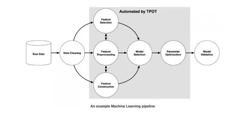
So the highlighted grey section in the image above is automated using TPOT. This automation is achieved using genetic algorithm.
So, without going deep into this, let’s directly try to implement it.
For using TPOT library, you first have to install some existing python libraries on which TPOT is build. So let us quickly install them.
- MATLAB CODE:-
clear all
close all
clc

%defining our search space
x = linspace(0,0.6,150);
y = linspace(0,0.6,150);

%creating a 2 dimensional mesh
[xx,yy] = meshgrid(x, y);
num_case = 80;

%evaluating the stalagmite function
for i = 1:length(xx)
    for j = 1:length(yy)
        input_vector(1)=xx(i,j);
        input_vector(2)=yy(i,j);
        f(i,j) = stalagmite(input_vector);
    end
end


%study one - static behaviour
tic
for i= 1:num_case
    [inputs, fopt(i)] = ga(@stalagmite,2);
    xopt(i) = inputs(1)
    yopt(i) = inputs(2)

end

studyone_time = toc

figure(1)
subplot(2,1,1)
hold on
surfc(x,y,-f)
shading interp
title('Unbound inputs')
xlabel('x value')
ylabel('y value')
plot3(xopt,yopt,-fopt,'marker','o','markersize',5,'markerfacecolor','r')

subplot(2,1,2)
plot(-fopt)
xlabel('Iterations')
ylabel('function maximum')

%study two - static behaviour with upper and lower bounds
tic
for i= 1:num_case
    [inputs, fopt(i)] = ga(@stalagmite,2,[],[],[],[],[0;0],[0.6;0.6]);
    xopt(i) = inputs(1);
    yopt(i) = inputs(2);

end

studytwo_time = toc

figure(2)
subplot(2,1,1)
hold on
surfc(x,y,-f)
shading interp
title('Bounded inputs')
xlabel('x value')
ylabel('y value')
plot3(xopt,yopt,-fopt,'marker','o','markersize',5,'markerfacecolor','r')

subplot(2,1,2)
plot(-fopt)
xlabel('Iterations')
ylabel('function maximum')

%study three - increasing ga itterations
options = optimoptions('ga')
options = optimoptions(options,'PopulationSize',200)
tic
for i= 1:num_case
    [inputs, fopt(i)] = ga(@stalagmite,2,[],[],[],[],[0;0],[0.6;0.6],[],[],options);
    xopt(i) = inputs(1);
    yopt(i) = inputs(2);

end

studyone_time = toc

figure(3)
subplot(2,1,1)
hold on
surfc(x,y,-f)
shading interp
xlabel('x value')
ylabel('y value')
plot3(xopt,yopt,-fopt,'marker','o','markersize',5,'markerfacecolor','r')
subplot(2,1,2)
plot(-fopt)
xlabel('Iterations')
ylabel('function maximum')
- FUNCTION CODE:-
function [f] = stalagmite(input_vector)
x = input_vector(1);
y = input_vector(2);

f1_x =(sin((5.1*pi*x)+0.5)).^6;
f1_y =(sin((5.1*pi*y)+0.5)).^6;

f2_x = exp(((-4*log(2))*(x-0.0667).^2)/0.64);
f2_y = exp(((-4*log(2))*(y-0.0667).^2)/0.64);

[f] = -(f1_x.*f1_y.*f2_x.*f2_y);
end
STEPS:
- The code starts with defining x and y as inputs using linspace.
- The combination of x and y value is taken in the stalagmite function.
- In the first study ga function runs at 80 irretations.plots of stalagmite and maximum values generated in each itteration is show.
- In the second study ga function is incorporated with lower and upper bounds and runs for 80 iterations.
- In the first study ga function is incorporated with lower and upper bounds along with the population size of 200.
RESULT:-
- STUDY ONE
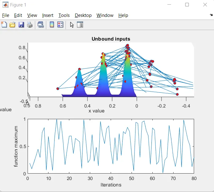
The solutions are not bounded so the ga will calculate all the possible maxima in X and Y cordinates.Time taken is 3.2951.
- STUDY TWO
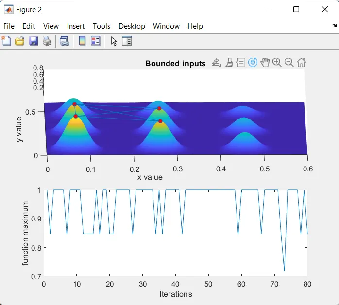
In the second study most of the maximum values obtained in each iteration varies between (1) to (0.7).This method narrow down the maximum values to 4 points.The time taken is 5.2020.
- STUDY THREE
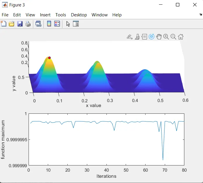
In the third study the global maximum obtained is accurate and is narrow down to a value of 0.999999 as show in the graph.